Thermally Induced Failure under Confined Cooling

Context

When a rock cools but cannot contract, it develops tensile stress. In a confined rock mass, this thermal stress combines with the existing in-situ stresses and may cause the rock to fail—even when pore pressure and external loading stay constant. This mechanism is responsible for thermal fracturing around cold-fluid injectors and caprock damage during CO₂ storage, among other phenomena.

This example simulates thermal contraction stresses using a one-dimensional thermo-mechanical problem. We compare two constitutive models subjected to the same cooling history:

Thermo-elastic rock (ElasticIsotropic): The induced stress increases indefinitely as the rock continues cooling.
Thermo-plastic rock (DruckerPrager): The induced stress is limited by the yield surface. Beyond a critical temperature drop, the rock fails and deforms plastically.

Both cases have closed-form solutions, making this example useful for verifying the thermo-mechanical coupling and the Drucker-Prager return mapping under thermal loading.

InputFile

This example uses no external input files. Everything required is contained within three GEOS input files located at:

inputFiles/thermoPoromechanics/ThermoMech_1DCooling_base.xml

inputFiles/thermoPoromechanics/ThermoElastic_1DCooling_fim_smoke.xml

inputFiles/thermoPoromechanics/ThermoDruckerPrager_1DCooling_fim_smoke.xml

Description of the case

We consider a seven-meter column discretized with 14 elements along the y direction, and a single element in the two other directions. The column is initially at a uniform temperature of 100 K, and is cooled down to 20 K following a linear ramp imposed over the whole domain.

The mechanical boundary conditions are the essential ingredient of the problem: the two ends of the column (yneg and ypos) are fixed along y, so the axial strain is prevented (ε_yy = 0), while the x and z directions are only restrained on one face each and are therefore free to deform. The lateral faces being traction-free, σ_xx = σ_zz = 0, and the only non-zero stress component is σ_yy.

$\varepsilon_{yy} = 0, \qquad \sigma_{xx} = \sigma_{zz} = 0$

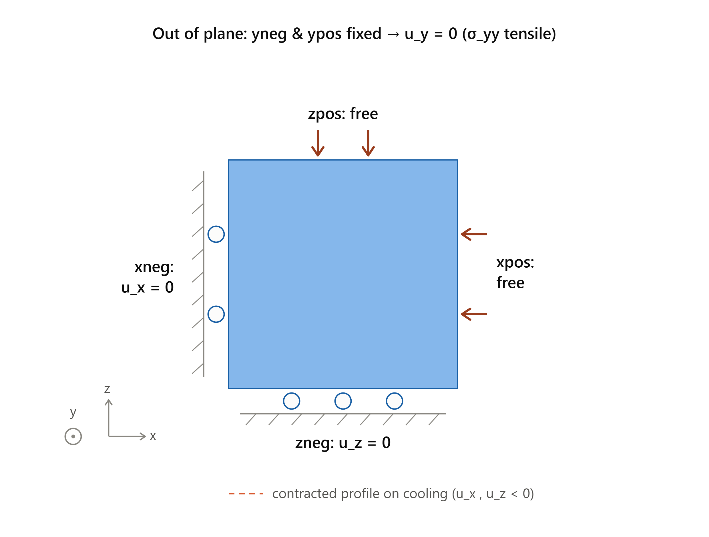
../../../../../../_images/xz_cross_section_uniaxial_stress.png — Fig. 83 Sketch of the confined column: both ends are fixed along `y`, while `x` and `z` are restrained on a single face each and remain free to deform.

    <FieldSpecification
      name="xconstraint"
      fieldName="totalDisplacement"
      component="0"
      objectPath="nodeManager"
      setNames="{ xneg }"/>

    <FieldSpecification
      name="yconstraint"
      fieldName="totalDisplacement"
      component="1"
      objectPath="nodeManager"
      setNames="{ yneg, ypos }"/>

    <FieldSpecification
      name="zconstraint"
      fieldName="totalDisplacement"
      component="2"
      objectPath="nodeManager"
      setNames="{ zneg }"/>

The cooling history is prescribed by a TableFunction applied to the temperature field. A short initial temperature plateau lets the mechanical equilibrium settle before the thermal loading starts.

    <TableFunction
      name="timeFunction"
      inputVarNames="{ time }"
      coordinates="{ 0, 1e-10, 100.0 }"
      values="{ 100.0, 100.0, 20.0 }"/>

The pore pressure is fixed to zero and the permeability is set to a negligible value ( $10^{-100}$ m²), so that no fluid flow takes place: the stress evolution is entirely thermo-mechanical, like in the analytical solution.

Constitutive models

The two cases differ only by the solid model. The thermo-elastic case uses an ElasticIsotropic solid, with a drained linear thermal expansion coefficient $\alpha = 3 \times 10^{-7}$ K^-1:

    <ElasticIsotropic
      name="rockSolid"
      defaultDensity="2700"
      defaultBulkModulus="0.5e9"
      defaultShearModulus="0.3e9"
      defaultDrainedLinearTEC="3e-7"/>

The thermo-plastic case uses the same elastic properties and thermal expansion coefficient, and adds a Drucker-Prager yield surface:

    <DruckerPrager
      name="rockSolid"
      defaultDensity="2700"
      defaultBulkModulus="0.5e9"
      defaultShearModulus="0.3e9"
      defaultCohesion="5e3"
      defaultFrictionAngle="15.27"
      defaultDilationAngle="0.0"
      defaultHardeningRate="0.0"
      defaultDrainedLinearTEC="3e-7"/>

Analytical solution

Thermo-elastic response. In this uniaxial stress state (σ_xx = σ_zz = 0), the axial strain is blocked (ε_yy = 0) and the thermo-elastic constitutive law reduces to

$\sigma_{yy} = -E \, \alpha \, \Delta T$

with $E = 9KG/(3K+G)$ the Young modulus. A cooling $\Delta T < 0$ therefore produces a tensile stress that grows linearly with the temperature drop, without any bound.

Onset of failure. The Drucker-Prager yield function implemented in GEOS reads

$F = Q + b \, P - c$

where $P = \mathrm{tr}(\sigma)/3$ is the mean stress and $Q$ the von Mises stress. The two coefficients are obtained from the friction angle $\varphi$ and the cohesion so that the cone passes through the triaxial compression corners of the Mohr-Coulomb surface:

$b = \frac{6 \sin \varphi}{3 - \sin \varphi}, \qquad c = \frac{6\, \mathrm{cohesion} \cos \varphi}{3 - \sin \varphi}$

For the uniaxial stress state of this problem, $Q = \sigma_{yy}$ and $P = \sigma_{yy}/3$ , so the yield condition $F = 0$ gives a closed-form cap on the thermally induced stress, and the corresponding critical cooling:

$\sigma_{f} = \frac{c}{1 + b/3}, \qquad \Delta T_{f} = -\frac{\sigma_{f}}{E \, \alpha}$

With the properties of this example, $\sigma_{f} = 8868$ Pa is reached after a cooling of only $\Delta T_{f} = -39.4$ K, that is, less than half of the imposed temperature drop. Beyond that point the rock deforms plastically and the stress stays on the yield surface.

Lateral displacement. Because the y direction is blocked while x and z are free, all the deformation shows up laterally, and this gives a second, kinematic check that is independent from the stress. In the elastic regime,

$\varepsilon_{xx} = \alpha \, \Delta T \left( 1 + \frac{\lambda}{2(\lambda + G)} \right)$

Once the yield surface is reached, plastic flow adds lateral strain while the stress stays put: the elasto-plastic column keeps contracting faster than the elastic one. Both branches are implemented in AnalyticalSol.py, which is the reference solution used below.

Running the case and post-processing

Both cases are run independently, each in its own directory:

geosx -i ThermoElastic_1DCooling_fim_smoke.xml
geosx -i ThermoDruckerPrager_1DCooling_fim_smoke.xml

Each run writes stressHistory.hdf5 and displacementHistory.hdf5 through the TimeHistory outputs. Those files are not stored in the repository; the curves shown below are extracted once, locally, into a small CSV file with:

python3 postprocess1DCooling.py -e <elastic_run_dir> -d <druckerPrager_run_dir>

The figure of this page is then generated at documentation build time from that CSV only.

Results

(Source code)

../../../../../../_images/plot1DCooling.png

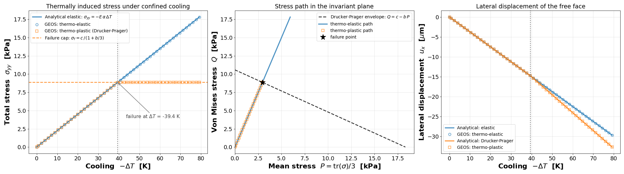
The figure on the left shows the stress induced by the confined cooling. Up to $-\Delta T \approx 39$ K the two models are indistinguishable and follow the elastic line $-E \alpha \Delta T$ exactly. Past that threshold, the elastic rock keeps accumulating tensile stress and reaches 17.8 kPa at the end of the cooling, whereas the Drucker-Prager rock yields and its stress saturates at the analytical cap $\sigma_{f}$ , matching to machine precision.

The figure in the middle explains the mechanism in the invariant plane. Because $\sigma_{xx} = \sigma_{zz} = 0$ , the loading path is the straight line $Q = 3P$ , whatever the amount of cooling. The elastic path simply crosses the Drucker-Prager envelope and keeps going, which is physically inadmissible; the elasto-plastic path stops on the envelope and slides along it.

The figure on the right shows the kinematic counterpart. Up to the failure threshold, the two columns contract identically. Beyond it, the roles reverse with respect to the stress plot: the elasto-plastic column, whose stress is now frozen, contracts more than the elastic one, reaching $-32.7$ against $-29.7$ µm. Plastic flow converts what would have been additional stress into additional strain. GEOS matches the analytical displacement of both branches to machine precision.

The practical consequence is that the safe amount of cooling is set by the strength of the rock, not by its stiffness alone: an elastic-only analysis of a cold injection would over-predict the stress by a factor of two here, under-predict the deformation, and miss the failure entirely.

To go further

Feedback on this example

For any feedback on this example, please submit a GitHub issue on the project’s GitHub page.