Verification of CO2 Core Flood Experiment with Buckley-Leverett Solution

Context

In this example, we simulate a CO2 core flood experiment representing immiscible transport of two-phase flow (CO2 and water) through porous media (Ekechukwu et al., 2022). This problem is solved using the multiphase flow solver in GEOS to obtain the temporal evolution of saturation along the flow direction, and verified against the Buckley-Leverett analytical solutions (Buckley and Leverett, 1942; Arabzai and Honma, 2013).

Input file

The xml input files for the test case are located at:

inputFiles/compositionalMultiphaseFlow/benchmarks/buckleyLeverettProblem/buckleyLeverett_base.xml
inputFiles/compositionalMultiphaseFlow/benchmarks/buckleyLeverettProblem/buckleyLeverett_benchmark.xml

Table files and a Python script for post-processing the simulation results are provided:

inputFiles/compositionalMultiphaseFlow/benchmarks/buckleyLeverettProblem/buckleyLeverett_table

src/docs/sphinx/advancedExamples/validationStudies/carbonStorage/buckleyLeverett/buckleyLeverettFigure.py

Description of the case

We model the immiscible displacement of brine by CO2 in a quasi one-dimensional domain that mimics a CO2 core flood experiment, as shown below. The domain is horizontal, homogeneous, isotropic and isothermal. Prior to injection, the domain is fully saturated with brine. To match the analytical example configuration, supercritical CO2 is injected from the inlet and a constant flow rate is imposed. To meet the requirements of immiscible transport in one-dimensional domain, we assume linear and horizontal flow, incompressible and immiscible phases, negligible capillary pressure and gravitational forces, and no poromechanical effects. Upon injection, the saturation front of the injected phase (supercritical CO2) forms a sharp leading edge and advances with time.

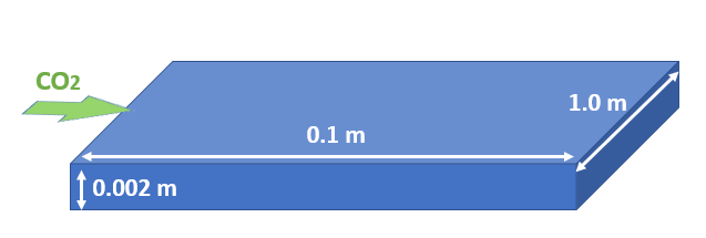
../../../../../../_images/sketch.png — Fig. 2 Sketch of the problem

We set up and solve a multiphase flow model to obtain the spatial and temporal solutions of phase saturations and pore pressures across the domain upon injection. Saturation profiles along the flow direction are evaluated and compared with their corresponding analytical solutions (Arabzai and Honma, 2013).

A power-law Brooks-Corey relation is used here to describe gas $k_{rg}$ and water $k_{rw}$ relative permeabilities:

$k_{rg} = {k_{rg}}^{0} { \left( {S_g}^{\star} \right) }^{n_g}$

$k_{rw} = {k_{rw}}^{0} { \left( {S_w}^{\star} \right) }^{n_w}$

where ${k_{rg}}^{0}$ and ${k_{rw}}^{0}$ are the maximum relative permeability of gas and water phase respectively; $n_g$ and $n_w$ are the Corey exponents; dimensionless volume fraction (saturation) of gas phase ${S_g}^{\star}$ and water phase ${S_w}^{\star}$ are given as:

${S_g}^{\star} = \frac{ S_g - S_{gr} }{1 - S_{gr} - S_{wr} }$

${S_w}^{\star} = \frac{ S_w - S_{wr} }{1 - S_{gr} - S_{wr} }$

where $S_{gr}$ and $S_{wr}$ are the residual gas and water saturation;

According to the Buckley–Leverett theory with constant fluid viscosity, the fractional flow of gas phase $f_g$ can be expressed as:

$f_g = \frac {\frac{k_{rg}}{\mu_g}} { \frac{k_{rg}}{\mu_g} + \frac{k_{rw}}{\mu_w}}$

where $\mu_g$ and $\mu_w$ represent the viscosity of gas and water phase respectively, assumed to be constant in this study.

The position of a particular saturation is given as a function of the injection time $t$ and the value of the derivative $\frac{df_g}{dS_g}$ at that saturation:

$x_{S_g} = \frac {Q_T t } { A \phi} { \left( \frac{df_g}{dS_g} \right) }$

where $Q_T$ is the total flow rate, $A$ is the area of the cross-section in the core sample, $\phi$ is the rock porosity. In addition, the abrupt saturation front is determined based on the tangent point on the fractional flow curve.

For this example, we focus on the Mesh, the Constitutive, and the FieldSpecifications tags.

Mesh

The mesh was created with the internal mesh generator and parametrized in the InternalMesh XML tag. It contains 1000x1x1 eight-node brick elements in the x, y, and z directions respectively. Such eight-node hexahedral elements are defined as C3D8 elementTypes, and their collection forms a mesh with one group of cell blocks named here cellBlock. The width of the domain should be large enough to ensure the formation of a one-dimension flow.

  <Mesh>
    <InternalMesh
      name="mesh"
      elementTypes="{ C3D8 }"
      xCoords="{ 0, 0.1 }"
      yCoords="{ 0, 0.00202683 }"
      zCoords="{ 0, 1 }"
      nx="{ 1000 }"
      ny="{ 1 }"
      nz="{ 1 }"
      cellBlockNames="{ cellBlock }"/>
  </Mesh>

Flow solver

The isothermal immiscible simulation is performed using the GEOS general-purpose multiphase flow solver. The multiphase flow solver, a solver of type CompositionalMultiphaseFVM called here compflow (more information on these solvers at Compositional Multiphase Flow Solver) is defined in the XML block CompositionalMultiphaseFVM:

  <Solvers>
    <CompositionalMultiphaseFVM
      name="compflow"
      logLevel="1"
      discretization="fluidTPFA"
      temperature="300"
      initialDt="0.001"
      useMass="1"
      targetRegions="{ region }">
      <NonlinearSolverParameters
        newtonTol="1.0e-6"
        newtonMaxIter="50"
        maxTimeStepCuts="2"
        lineSearchMaxCuts="2"/>
      <LinearSolverParameters
        solverType="direct"
        directParallel="0"  
        logLevel="0"/>
    </CompositionalMultiphaseFVM>
  </Solvers>

We use the targetRegions attribute to define the regions where the flow solver is applied. Here, we only simulate fluid flow in one region named as region. We specify the discretization method (fluidTPFA, defined in the NumericalMethods section), and the initial reservoir temperature (temperature="300").

Constitutive laws

This benchmark example involves an immiscible, incompressible, two-phase model, whose fluid rheology and permeability are specified in the Constitutive section. The best approach to represent this fluid behavior in GEOS is to use the DeadOilFluid model in GEOS.

  <Constitutive>
    <CompressibleSolidConstantPermeability
      name="rock"
      solidModelName="nullSolid"
      porosityModelName="rockPorosity"
      permeabilityModelName="rockPerm"/>

    <NullModel
      name="nullSolid"/>

    <PressurePorosity
      name="rockPorosity"
      defaultReferencePorosity="0.2"
      referencePressure="1e7"
      compressibility="1.0e-15"/>

    <ConstantPermeability
      name="rockPerm"
      permeabilityComponents="{ 9.0e-13, 9.0e-13, 9.0e-13}"/>   

    <BrooksCoreyRelativePermeability
      name="relperm"
      phaseNames="{ gas, water }"
      phaseMinVolumeFraction="{ 0.0, 0.0 }"
      phaseRelPermExponent="{ 3.5, 3.5 }"
      phaseRelPermMaxValue="{ 1.0, 1.0 }"/>
    
    <DeadOilFluid
      name="fluid"
      phaseNames="{ gas, water }"
      surfaceDensities="{ 280.0, 992.0 }"
      componentMolarWeight="{ 44e-3, 18e-3 }"
      tableFiles="{ buckleyLeverett_table/pvdg.txt, buckleyLeverett_table/pvtw.txt }"/>
  </Constitutive>

Constant fluid densities and viscosities are given in the external tables for both phases. The formation volume factors are set to 1 for incompressible fluids. The relative permeability for both phases are modeled with the power-law correlations BrooksCoreyRelativePermeability (more information at Brooks-Corey relative permeability model), as shown below. Capillary pressure is assumed to be negligible.

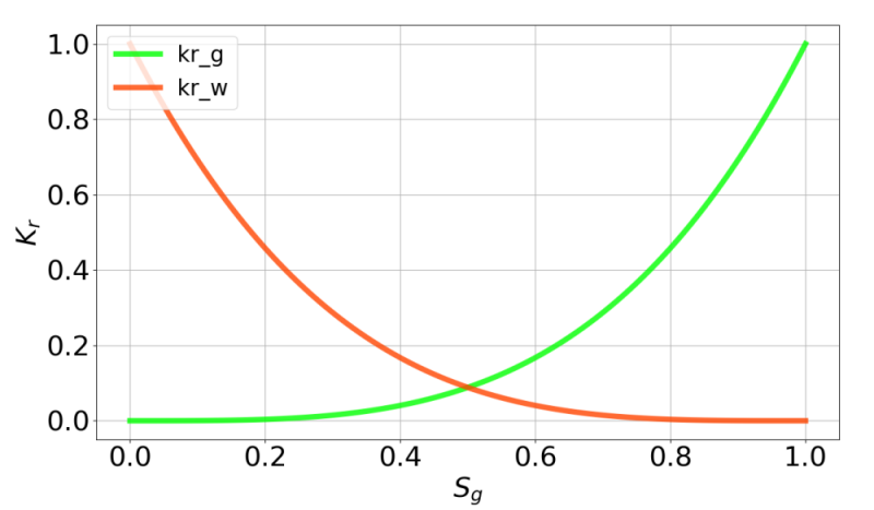
../../../../../../_images/brooksCoreyRelativePermeability.png — Fig. 3 Relative permeabilities of both phases

All constitutive parameters such as density, viscosity, and permeability are specified in the International System of Units.

Time history function

In the Tasks section, PackCollection tasks are defined to collect time history information from fields. Either the entire field or specified named sets of indices in the field can be collected. In this example, phaseVolumeFractionCollection is specified to output the time history of phase saturations fieldName="phaseVolumeFraction" across the computational domain.

  <Tasks>
    <PackCollection
      name="phaseVolumeFractionCollection"
      objectPath="ElementRegions/region/cellBlock"
      fieldName="phaseVolumeFraction"/>
  </Tasks>

This task is triggered using the Event manager with a PeriodicEvent defined for the recurring tasks. GEOS writes one file named after the string defined in the filename keyword, formatted as a HDF5 file (saturationHistory.hdf5). The TimeHistory file contains the collected time history information from the specified time history collector. This file includes datasets for the simulation time, element center, and the time history information for both phases. A Python script is prepared to read and plot any specified subset of the time history data for verification and visualization.

Initial and boundary conditions

The next step is to specify fields, including:

The initial value (the pore pressure and phase saturations have to be initialized)

The boundary conditions (fluid injection rates and controls on the fluid outlet have to be set)

In this example, the domain is initially saturated with brine in a uniform pressure field. The component attribute of the FieldSpecification XML block must use the order in which the phaseNames have been defined in the DeadOilFluid XML block. In other words, component=0 is used to initialize the gas global component fraction and component=1 is used to initialize the water global component fraction, because we previously set phaseNames="{gas, water}" in the DeadOilFluid XML block.

A mass injection rate SourceFlux (scale="-0.00007") of pure CO2 (component="0") is applied at the fluid inlet, named source. The value given for scale is $Q_T \rho_g$ . Pressure and composition controls at the fluid outlet (sink) are also specified. The setNames="{ source } and setNames="{ sink }" are defined using the Box XML tags of the Geometry section.

These boundary conditions are set up through the FieldSpecifications section.

  <FieldSpecifications>
    <FieldSpecification
      name="initialPressure"
      initialCondition="1"
      setNames="{ all }"
      objectPath="ElementRegions"
      fieldName="pressure"
      scale="1e7"/>

    <FieldSpecification
      name="initialComposition_gas"
      initialCondition="1"
      setNames="{ all }"
      objectPath="ElementRegions"
      fieldName="globalCompFraction"
      component="0"
      scale="0.001"/>

    <FieldSpecification
      name="initialComposition_water"
      initialCondition="1"
      setNames="{ all }"
      objectPath="ElementRegions"
      fieldName="globalCompFraction"
      component="1"
      scale="0.999"/>

    <SourceFlux
      name="sourceTerm"
      objectPath="ElementRegions"
      scale="-0.00007"
      component="0"
      setNames="{ source }"/>

    <FieldSpecification
      name="sinkTermPressure"
      objectPath="faceManager"
      fieldName="pressure"
      scale="1e7"
      setNames="{ sink }"/>

    <FieldSpecification
      name="sinkTermTemperature"
      objectPath="faceManager"
      fieldName="temperature"
      scale="300"
      setNames="{ sink }"/>

    <FieldSpecification
      name="sinkTermComposition_gas"
      setNames="{ sink }"
      objectPath="faceManager"
      fieldName="globalCompFraction"
      component="0"
      scale="0.001"/>

    <FieldSpecification
      name="sinkTermComposition_water"
      setNames="{ sink }"
      objectPath="faceManager"
      fieldName="globalCompFraction"
      component="1"
      scale="0.999"/>    
  </FieldSpecifications>

The parameters used in the simulation are summarized in the following table, and specified in the Constitutive and FieldSpecifications sections.

Symbol	Parameter	Unit	Value
${k_{rg}}^{0}$	Max Relative Permeability of Gas	[-]	1.0
${k_{rw}}^{0}$	Max Relative Permeability of Water	[-]	1.0
$n_g$	Corey Exponent of Gas	[-]	3.5
$n_w$	Corey Exponent of Water	[-]	3.5
$S_{gr}$	Residual Gas Saturation	[-]	0.0
$S_{wr}$	Residual Water Saturation	[-]	0.0
$\phi$	Porosity	[-]	0.2
$\kappa$	Matrix Permeability	[m²]	9.0*10^-13
$\mu_g$	Gas Viscosity	[Pa s]	2.3*10^-5
$\mu_w$	Water Viscosity	[Pa s]	5.5*10^-4
$Q_T$	Total Flow Rate	[m³/s]	2.5*10^-7
$D_L$	Domain Length	[m]	0.1
$D_W$	Domain Width	[m]	1.0
$D_T$	Domain Thickness	[m]	0.002

Inspecting results

We request VTK-format output files and use Paraview to visualize the results. The following figure shows the distribution of phase saturations and pore pressures in the computational domain at $t=70 s$ .

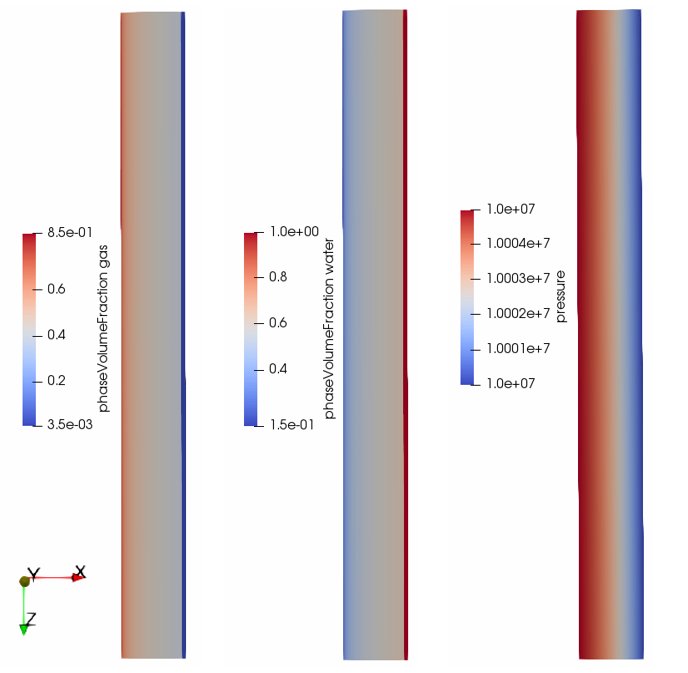
../../../../../../_images/contour.png — Fig. 4 Simulation results of phase saturations and pore pressure

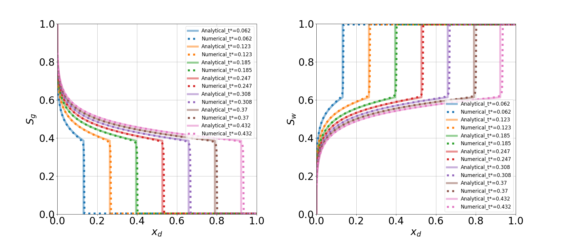
Two following dimensionless terms are defined when comparing the numerical solution with the analytical solutions:

${t}^{\star} = \frac {Q_T t } { A D_L \phi}$

$x_d = \frac { x_{S_g} } { D_L }$

The figure below compares the results from GEOS (dashed curves) and the corresponding analytical solution (solid curves) for the change of gas saturation ( $S_g$ ) and water saturation ( $S_w$ ) along the flow direction.

GEOS reliably captures the immiscible transport of two phase flow (CO2 and water). GEOS matches the analytical solutions in the formation and the progress of abrupt fronts in the saturation profiles.

(Source code)

../../../../../../_images/buckleyLeverettFigure.png

To go further

Feedback on this example

For any feedback on this example, please submit a GitHub issue on the project’s GitHub page.