Multiphase Flow with Wells
Context
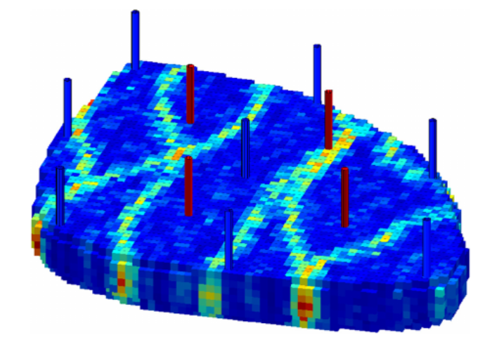
In this example, we build on the concepts presented in Multiphase Flow to show how to set up a multiphase water injection problem with wells in the three-dimensional Egg model. The twelve wells (four producers and eight injectors) are placed according to the description of the original test case.
Objectives
In this example, we re-use many GEOS features already presented in Multiphase Flow, but we now focus on:
how to import an external mesh with embedded geological properties (permeability) in the VTK format (
.vtu),how to set up the wells.
Input file
This example is based on the XML file located at
../../../../../inputFiles/compositionalMultiphaseWell/benchmarks/Egg/deadOilEgg_benchmark.xml
The mesh file corresponding to the Egg model is stored in the GEOSDATA repository. Therefore, you must first download the GEOSDATA repository in the same folder as the GEOS repository to run this test case.
Note
GEOSDATA is a separate repository in which we store large mesh files in order to keep the main GEOS repository lightweight.
The XML file considered here follows the typical structure of the GEOS input files:
Coupling the flow solver with wells
In GEOS, the simulation of reservoir flow with wells is set up by combining three solvers listed and parameterized in the Solvers XML block of the input file. We introduce separately a flow solver and a well solver acting on different regions of the domain—respectively, the reservoir region and the well regions. To drive the simulation and bind these single-physics solvers, we also specify a coupling solver between the reservoir flow solver and the well solver. This coupling of single-physics solvers is the generic approach used in GEOS to define multiphysics problems. It is illustrated in Poromechanics for a poroelastic test case.
The three solvers employed in this example are:
the single-physics reservoir flow solver, a solver of type CompositionalMultiphaseFVM named
compositionalMultiphaseFlow(more information on this solver at Compositional Multiphase Flow Solver),the single-physics well solver, a solver of type CompositionalMultiphaseWell named
compositionalMultiphaseWell(more information on this solver at Compositional Multiphase Well Solver),the coupling solver that binds the two single-physics solvers above, an object of type CompositionalMultiphaseReservoir named
coupledFlowAndWells.
The Solvers XML block is shown below.
The coupling solver points to the two single-physics solvers using the attributes
flowSolverName and wellSolverName.
These names can be chosen by the user and are not imposed by GEOS.
The flow solver is applied to the reservoir and the well solver is applied to the wells,
as specified by their respective targetRegions attributes.
The simulation is fully coupled and driven by the coupled solver. Therefore, the time stepping
information (here, initialDt, but there may be other parameters used to fine-tune the time
stepping strategy), the nonlinear solver parameters, and the linear solver parameters must be
specified at the level of the coupling solver.
There is no need to specify these parameters at the level of the single-physics solvers.
Any solver information specified in the single-physics XML blocks will not be taken into account.
Note
It is worth repeating the logLevel="1" parameter at the level of the well solver to make sure that a notification is issued when the well control is switched (from rate control to BHP control, for instance).
Here, we instruct GEOS to perform at most newtonMaxIter = "10" Newton iterations.
GEOS will adjust the time step size as follows:
if the Newton solver converges in
timeStepIncreaseIterLimit x newtonMaxIter = 5iterations or fewer, GEOS will double the time step size for the next time step,if the Newton solver converges in
timeStepDecreaseIterLimit x newtonMaxIter = 8iterations or more, GEOS will reduce the time step size for the next time step by a factortimestepCutFactor = 0.1,if the Newton solver fails to converge in
newtonMaxIter = 10, GEOS will cut the time step size by a factortimestepCutFactor = 0.1and restart from the previous converged time step.
The maximum number of time step cuts is specified by the attribute maxTimeStepCuts.
Note that a backtracking line search can be activated by setting the attribute lineSearchAction to Attempt or Require.
If lineSearchAction = "Attempt", we accept the nonlinear iteration even if the line search does not reduce the residual norm.
If lineSearchAction = "Require", we cut the time step if the line search does not reduce the residual norm.
Note
To use the linear solver options of this example, you need to ensure that GEOS is configured to use the Hypre linear solver package.
  <Solvers>
    <CompositionalMultiphaseReservoir
      name="coupledFlowAndWells"
      flowSolverName="compositionalMultiphaseFlow"
      wellSolverName="compositionalMultiphaseWell"
      logLevel="1"
      initialDt="1e4"
      targetRegions="{ reservoir, wellRegion1, wellRegion2, wellRegion3, wellRegion4, wellRegion5, wellRegion6, wellRegion7, wellRegion8, wellRegion9, wellRegion10, wellRegion11, wellRegion12 }">
      <NonlinearSolverParameters
        newtonTol="1.0e-4"
        newtonMaxIter="25"
        timeStepDecreaseIterLimit="0.9"
        timeStepIncreaseIterLimit="0.6"
        timeStepCutFactor="0.1"
        maxTimeStepCuts="10"
        lineSearchAction="None"/>
      <LinearSolverParameters
        solverType="fgmres"
        preconditionerType="mgr"
        krylovTol="1e-4"
        krylovAdaptiveTol="1"
        krylovWeakestTol="1e-2"
        logLevel="1"/>
    </CompositionalMultiphaseReservoir>

    <CompositionalMultiphaseFVM
      name="compositionalMultiphaseFlow"
      targetRegions="{ reservoir }"
      discretization="fluidTPFA"
      temperature="297.15"
      maxCompFractionChange="0.3"
      logLevel="1"
      useMass="1"/>

    <CompositionalMultiphaseWell
      name="compositionalMultiphaseWell"
      targetRegions="{ wellRegion1, wellRegion2, wellRegion3, wellRegion4, wellRegion5, wellRegion6, wellRegion7, wellRegion8, wellRegion9, wellRegion10, wellRegion11, wellRegion12 }"
      maxCompFractionChange="0.5"
      logLevel="1"
      useMass="1">
      <WellControls
        name="wellControls1"
        type="producer"
        control="BHP"
        referenceElevation="28"
        targetBHP="3.9e7"
        targetPhaseRate="1e6"
        targetPhaseName="oil"/>
      <WellControls
        name="wellControls2"
        type="producer"
        control="BHP"
        referenceElevation="28"
        targetBHP="3.9e7"
        targetPhaseRate="1e6"
        targetPhaseName="oil"/>
Mesh definition and well geometry
In the presence of wells, the Mesh block of the XML input file includes two parts:
a sub-block VTKMesh defining the reservoir mesh (see Tutorial 2: External Meshes for more on this),
a collection of sub-blocks defining the geometry of the wells.
The reservoir mesh is imported from a .vtu file that contains the mesh geometry
and also includes the permeability values in the x, y, and z directions.
These quantities must be specified using the metric unit system, i.e., in meters
for the well geometry and square meters for the permeability field.
We note that the mesh file only contains active cells, so there is no keyword
needed in the XML file to define them.
  <Mesh>
    <VTKMesh
      name="mesh"
      file="../../../../../GEOSDATA/DataSets/Egg/egg.vtu"
      fieldsToImport="{ PERM }"
      fieldNamesInGEOS="{ rockPerm_permeability }">

      <InternalWell
        name="wellProducer1"
        wellRegionName="wellRegion1"
        wellControlsName="wellControls1"
        polylineNodeCoords="{ { 124, 340, 28 },
                              { 124, 340, 0 } }"
        polylineSegmentConn="{ { 0, 1 } }"
        radius="0.1"
        numElementsPerSegment="7">
        <Perforation
          name="producer1_perf1"
          distanceFromHead="2"/>
        <Perforation
          name="producer1_perf2"
          distanceFromHead="6"/>
        <Perforation
          name="producer1_perf3"
          distanceFromHead="10"/>
        <Perforation
          name="producer1_perf4"
          distanceFromHead="14"/>
        <Perforation
          name="producer1_perf5"
          distanceFromHead="18"/>
        <Perforation
          name="producer1_perf6"
          distanceFromHead="22"/>
        <Perforation
          name="producer1_perf7"
          distanceFromHead="26"/>
      </InternalWell>

      <InternalWell
        name="wellProducer2"
        wellRegionName="wellRegion2"
        wellControlsName="wellControls2"
        polylineNodeCoords="{ { 276, 316, 28 },
                              { 276, 316, 0 } }"
        polylineSegmentConn="{ { 0, 1 } }"
        radius="0.1"
        numElementsPerSegment="7">
        <Perforation
          name="producer2_perf1"
          distanceFromHead="2"/>
        <Perforation
          name="producer2_perf2"
          distanceFromHead="6"/>
        <Perforation
          name="producer2_perf3"
          distanceFromHead="10"/>
        <Perforation
          name="producer2_perf4"
          distanceFromHead="14"/>
        <Perforation
          name="producer2_perf5"
          distanceFromHead="18"/>
        <Perforation
          name="producer2_perf6"
          distanceFromHead="22"/>
        <Perforation
          name="producer2_perf7"
          distanceFromHead="26"/>
      </InternalWell>
InternalWell sub-blocks
Each well is defined internally (i.e., not imported from a file) in a separate InternalWell
XML sub-block. An InternalWell sub-block must point to the region corresponding to this well using the attribute
wellRegionName, and to the control of this well using the attribute wellControl.
Each well is defined using a vertical polyline going through the seven layers of the mesh with a perforation in each layer. The well placement implemented here follows the pattern of the original test case. The well geometry must be specified in meters.
The location of the perforations is found internally using the linear distance along the wellbore
from the top of the well specified by the attribute distanceFromHead.
It is the responsibility of the user to make sure that there is a perforation in the bottom cell
of the well mesh otherwise an error will be thrown and the simulation will terminate.
For each perforation, the well transmissibility factors employed to compute the perforation rates are calculated
internally using the Peaceman formulation.
VTKWell sub-blocks
Each well is loaded from a file in a separate VTKWell
XML sub-block. A VTKWell sub-block must point to the region corresponding to this well using the attribute
wellRegionName, and to the control of this well using the attribute wellControl.
Each well is defined using a vertical VTK polyline going through the seven layers of the mesh with a perforation in each layer. The well placement implemented here follows the pattern of the original test case. The well geometry must be specified in meters.
The location of perforations is found internally using the linear distance along the wellbore
from the top of the well specified by the attribute distanceFromHead.
It is the responsibility of the user to make sure that there is a perforation in the bottom cell
of the well mesh otherwise an error will be thrown and the simulation will terminate.
For each perforation, the well transmissibility factors employed to compute the perforation rates are calculated
internally using the Peaceman formulation.
  <Mesh>
    <VTKMesh
      name="mesh"
      file="../../../../../GEOSDATA/DataSets/Egg/egg.vtu"
      fieldsToImport="{ PERM }"
      fieldNamesInGEOS="{ rockPerm_permeability }">

      <VTKWell
        name="wellProducer1"
        wellRegionName="wellRegion1"
        wellControlsName="wellControls1"
        file="../../../../../GEOSDATA/DataSets/Egg/wellProducer1.vtk"
        radius="0.1"
        numElementsPerSegment="7">
        <Perforation
          name="producer1_perf1"
          distanceFromHead="2"/>
        <Perforation
          name="producer1_perf2"
          distanceFromHead="6"/>
        <Perforation
          name="producer1_perf3"
          distanceFromHead="10"/>
        <Perforation
          name="producer1_perf4"
          distanceFromHead="14"/>
        <Perforation
          name="producer1_perf5"
          distanceFromHead="18"/>
        <Perforation
          name="producer1_perf6"
          distanceFromHead="22"/>
        <Perforation
          name="producer1_perf7"
          distanceFromHead="26"/>
      </VTKWell>

      <VTKWell
        name="wellProducer2"
        wellRegionName="wellRegion2"
        wellControlsName="wellControls2"
        file="../../../../../GEOSDATA/DataSets/Egg/wellProducer2.vtk"
        radius="0.1"
        numElementsPerSegment="7">
        <Perforation
          name="producer2_perf1"
          distanceFromHead="2"/>
        <Perforation
          name="producer2_perf2"
          distanceFromHead="6"/>
        <Perforation
          name="producer2_perf3"
          distanceFromHead="10"/>
        <Perforation
          name="producer2_perf4"
          distanceFromHead="14"/>
        <Perforation
          name="producer2_perf5"
          distanceFromHead="18"/>
        <Perforation
          name="producer2_perf6"
          distanceFromHead="22"/>
        <Perforation
          name="producer2_perf7"
          distanceFromHead="26"/>
      </VTKWell>
Events
In the Events XML block, we specify four types of PeriodicEvents.
The periodic event named solverApplications notifies GEOS that the
coupled solver coupledFlowAndWells has to be applied to its target
regions (here, reservoir and wells) at every time step.
The time stepping strategy has been fully defined in the CompositionalMultiphaseReservoir
coupling block using the initialDt attribute and the NonlinearSolverParameters
nested block.
We also define an output event instructing GEOS to write out .vtk files at the time frequency specified
by the attribute timeFrequency.
Here, we choose to output the results using the VTK format (see Tutorial 2: External Meshes
for a example that uses the Silo output file format).
The target attribute must point to the VTK sub-block of the Outputs
block defined at the end of the XML file by its user-specified name (here, vtkOutput).
We define the events involved in the collection and output of well production rates following the procedure defined in Tasks Manager.
The time-history collection events trigger the collection of well rates at the desired frequency, while the time-history output events trigger the output of HDF5 files containing the time series.
These events point by name to the corresponding blocks of the Tasks and Outputs XML blocks. Here, these names are wellRateCollection1 and timeHistoryOutput1.
  <Events
    maxTime="1.5e7">
    <PeriodicEvent
      name="vtk"
      timeFrequency="2e6"
      target="/Outputs/vtkOutput"/>

    <PeriodicEvent
      name="timeHistoryOutput1"
      timeFrequency="1.5e7"
      target="/Outputs/timeHistoryOutput1"/>

    <PeriodicEvent
      name="timeHistoryOutput2"
      timeFrequency="1.5e7"
      target="/Outputs/timeHistoryOutput2"/>

    <PeriodicEvent
      name="timeHistoryOutput3"
      timeFrequency="1.5e7"
      target="/Outputs/timeHistoryOutput3"/>

    <PeriodicEvent
      name="timeHistoryOutput4"
      timeFrequency="1.5e7"
      target="/Outputs/timeHistoryOutput4"/>

    <PeriodicEvent
      name="solverApplications"
      maxEventDt="5e5"
      target="/Solvers/coupledFlowAndWells"/>

    <PeriodicEvent
      name="timeHistoryCollection1"
      timeFrequency="1e6"
      target="/Tasks/wellRateCollection1"/>

    <PeriodicEvent
      name="timeHistoryCollection2"
      timeFrequency="1e6"
      target="/Tasks/wellRateCollection2"/>

    <PeriodicEvent
      name="timeHistoryCollection3"
      timeFrequency="1e6"
      target="/Tasks/wellRateCollection3"/>

    <PeriodicEvent
      name="timeHistoryCollection4"
      timeFrequency="1e6"
      target="/Tasks/wellRateCollection4"/>

    <PeriodicEvent
      name="restarts"
      timeFrequency="7.5e6"
      targetExactTimestep="0"
      target="/Outputs/restartOutput"/>

  </Events>
Numerical methods
In the NumericalMethods XML block, we instruct GEOS to use a TPFA (Two-Point Flux Approximation) finite-volume
numerical scheme.
This part is similar to the corresponding section of Multiphase Flow, and has been adapted to match the specifications of the Egg model.
  <NumericalMethods>
    <FiniteVolume>
      <TwoPointFluxApproximation
        name="fluidTPFA"/>
    </FiniteVolume>
  </NumericalMethods>
Reservoir and well regions
In this section of the input file, we follow the procedure described in Multiphase Flow for the definition of the reservoir region with multiphase constitutive models.
We associate a CellElementRegion named reservoir to the reservoir mesh.
Since we have imported a mesh with only one region, we can set cellBlocks to { * }
(we could also set cellBlocks to { hexahedra } as the mesh has only hexahedral cells).
We also associate a WellElementRegion to each well. As the CellElementRegion,
it contains a materialList that must point (by name) to the constitutive models
defined in the Constitutive XML block.
  <ElementRegions>
    <CellElementRegion
      name="reservoir"
      cellBlocks="{ * }"
      materialList="{ fluid, rock, relperm }"/>

    <WellElementRegion
      name="wellRegion1"
      materialList="{ fluid }"/>

    <WellElementRegion
      name="wellRegion2"
      materialList="{ fluid }"/>
Constitutive models
The CompositionalMultiphaseFVM physics solver relies on at least four types of constitutive models listed in the Constitutive XML block:
a fluid model describing the thermodynamics behavior of the fluid mixture,
a relative permeability model,
a rock permeability model,
a rock porosity model.
All the parameters must be provided using the SI unit system.
This part is identical to that of Multiphase Flow.
  <Constitutive>
    <DeadOilFluid
      name="fluid"
      phaseNames="{ oil, water }"
      surfaceDensities="{ 848.9, 1025.2 }"
      componentMolarWeight="{ 114e-3, 18e-3 }"
      tableFiles="{ pvdo.txt, pvtw.txt }"/>

    <BrooksCoreyRelativePermeability
      name="relperm"
      phaseNames="{ oil, water }"
      phaseMinVolumeFraction="{ 0.1, 0.2 }"
      phaseRelPermExponent="{ 4.0, 3.0 }"
      phaseRelPermMaxValue="{ 0.8, 0.75 }"/>

    <CompressibleSolidConstantPermeability
      name="rock"
      solidModelName="nullSolid"
      porosityModelName="rockPorosity"
      permeabilityModelName="rockPerm"/>

    <NullModel
      name="nullSolid"/>

    <PressurePorosity
      name="rockPorosity"
      defaultReferencePorosity="0.2"
      referencePressure="0.0"
      compressibility="1.0e-13"/>

    <ConstantPermeability
      name="rockPerm"
      permeabilityComponents="{ 1.0e-12, 1.0e-12, 1.0e-12 }"/>
  </Constitutive>
Initial conditions
We are ready to specify the reservoir initial conditions of the problem in the FieldSpecifications XML block. The well variables do not have to be initialized here since they will be defined internally.
The formulation of the CompositionalMultiphaseFVM physics solver (documented
at Compositional Multiphase Flow Solver) requires the definition of the initial pressure field
and initial global component fractions.
We define here a uniform pressure field that does not satisfy the hydrostatic equilibrium,
but a hydrostatic initialization of the pressure field is possible using Functions:.
For the initialization of the global component fractions, we remind the user that their component
attribute (here, 0 or 1) is used to point to a specific entry of the phaseNames attribute
in the DeadOilFluid block.
Note that we also define the uniform porosity field here since it is not included in the mesh file imported by the VTKMesh.
  <FieldSpecifications>
    <FieldSpecification
      name="initialPressure"
      initialCondition="1"
      setNames="{ all }"
      objectPath="ElementRegions/reservoir/hexahedra"
      fieldName="pressure"
      scale="4e7"/>

    <FieldSpecification
      name="initialComposition_oil"
      initialCondition="1"
      setNames="{ all }"
      objectPath="ElementRegions/reservoir/hexahedra"
      fieldName="globalCompFraction"
      component="0"
      scale="0.9"/>

    <FieldSpecification
      name="initialComposition_water"
      initialCondition="1"
      setNames="{ all }"
      objectPath="ElementRegions/reservoir/hexahedra"
      fieldName="globalCompFraction"
      component="1"
      scale="0.1"/>
  </FieldSpecifications>
Outputs
In this section, we request an output of the results in VTK format and an output of the rates for each producing well. Note that the name defined here must match the name used in the Events XML block to define the output frequency.
  <Outputs>
    <VTK
      name="vtkOutput"/>

    <TimeHistory
      name="timeHistoryOutput1"
      sources="{ /Tasks/wellRateCollection1 }"
      filename="wellRateHistory1"/>

    <TimeHistory
      name="timeHistoryOutput2"
      sources="{ /Tasks/wellRateCollection2 }"
      filename="wellRateHistory2"/>

    <TimeHistory
      name="timeHistoryOutput3"
      sources="{ /Tasks/wellRateCollection3 }"
      filename="wellRateHistory3"/>

    <TimeHistory
      name="timeHistoryOutput4"
      sources="{ /Tasks/wellRateCollection4 }"
      filename="wellRateHistory4"/>

    <Restart
      name="restartOutput"/>

  </Outputs>
Tasks
In the Events block, we have defined four events requesting that a task periodically collects the rate for each producing well.
This task is defined here, in the PackCollection XML sub-block of the Tasks block.
The task contains the path to the object on which the field to collect is registered (here, a WellElementSubRegion) and the name of the field (here, wellElementMixtureConnectionRate).
The details of the history collection mechanism can be found in Tasks Manager.
  <Tasks>
    <PackCollection
      name="wellRateCollection1"
      objectPath="ElementRegions/wellRegion1/wellRegion1UniqueSubRegion"
      fieldName="wellElementMixtureConnectionRate"/>

    <PackCollection
      name="wellRateCollection2"
      objectPath="ElementRegions/wellRegion2/wellRegion2UniqueSubRegion"
      fieldName="wellElementMixtureConnectionRate"/>

    <PackCollection
      name="wellRateCollection3"
      objectPath="ElementRegions/wellRegion3/wellRegion3UniqueSubRegion"
      fieldName="wellElementMixtureConnectionRate"/>

    <PackCollection
      name="wellRateCollection4"
      objectPath="ElementRegions/wellRegion4/wellRegion4UniqueSubRegion"
      fieldName="wellElementMixtureConnectionRate"/>
  </Tasks>
All elements are now in place to run GEOS.
Running GEOS
The first few lines appearing to the console are indicating that the XML elements are read and registered correctly:
Adding Mesh: VTKMesh, mesh
Adding Mesh: InternalWell, wellProducer1
Adding Mesh: InternalWell, wellProducer2
Adding Mesh: InternalWell, wellProducer3
Adding Mesh: InternalWell, wellProducer4
Adding Mesh: InternalWell, wellInjector1
Adding Mesh: InternalWell, wellInjector2
Adding Mesh: InternalWell, wellInjector3
Adding Mesh: InternalWell, wellInjector4
Adding Mesh: InternalWell, wellInjector5
Adding Mesh: InternalWell, wellInjector6
Adding Mesh: InternalWell, wellInjector7
Adding Mesh: InternalWell, wellInjector8
Adding Solver of type CompositionalMultiphaseReservoir, named coupledFlowAndWells
Adding Solver of type CompositionalMultiphaseFVM, named compositionalMultiphaseFlow
Adding Solver of type CompositionalMultiphaseWell, named compositionalMultiphaseWell
Adding Event: PeriodicEvent, vtk
Adding Event: PeriodicEvent, timeHistoryOutput1
Adding Event: PeriodicEvent, timeHistoryOutput2
Adding Event: PeriodicEvent, timeHistoryOutput3
Adding Event: PeriodicEvent, timeHistoryOutput4
Adding Event: PeriodicEvent, solverApplications
Adding Event: PeriodicEvent, timeHistoryCollection1
Adding Event: PeriodicEvent, timeHistoryCollection2
Adding Event: PeriodicEvent, timeHistoryCollection3
Adding Event: PeriodicEvent, timeHistoryCollection4
Adding Event: PeriodicEvent, restarts
Adding Output: VTK, vtkOutput
Adding Output: TimeHistory, timeHistoryOutput1
Adding Output: TimeHistory, timeHistoryOutput2
Adding Output: TimeHistory, timeHistoryOutput3
Adding Output: TimeHistory, timeHistoryOutput4
Adding Output: Restart, restartOutput
Adding Object CellElementRegion named reservoir from ObjectManager::Catalog.
Adding Object WellElementRegion named wellRegion1 from ObjectManager::Catalog.
Adding Object WellElementRegion named wellRegion2 from ObjectManager::Catalog.
Adding Object WellElementRegion named wellRegion3 from ObjectManager::Catalog.
Adding Object WellElementRegion named wellRegion4 from ObjectManager::Catalog.
Adding Object WellElementRegion named wellRegion5 from ObjectManager::Catalog.
Adding Object WellElementRegion named wellRegion6 from ObjectManager::Catalog.
Adding Object WellElementRegion named wellRegion7 from ObjectManager::Catalog.
Adding Object WellElementRegion named wellRegion8 from ObjectManager::Catalog.
Adding Object WellElementRegion named wellRegion9 from ObjectManager::Catalog.
Adding Object WellElementRegion named wellRegion10 from ObjectManager::Catalog.
Adding Object WellElementRegion named wellRegion11 from ObjectManager::Catalog.
Adding Object WellElementRegion named wellRegion12 from ObjectManager::Catalog.
This is followed by the creation of the 18553 hexahedral cells of the imported mesh. At this point, we are done with the case set-up and the code steps into the execution of the simulation itself:
Time: 0s, dt:10000s, Cycle: 0
    Attempt:  0, ConfigurationIter:  0, NewtonIter:  0
    ( Rflow ) = ( 1.01e+01 ) ;     ( Rwell ) = ( 4.96e+00 ) ;     ( R ) = ( 1.13e+01 ) ;
    Attempt:  0, ConfigurationIter:  0, NewtonIter:  1
    ( Rflow ) = ( 1.96e+00 ) ;     ( Rwell ) = ( 8.07e-01 ) ;     ( R ) = ( 2.12e+00 ) ;
    Last LinSolve(iter,res) = (  44, 8.96e-03 ) ;
    Attempt:  0, ConfigurationIter:  0, NewtonIter:  2
    ( Rflow ) = ( 4.14e-01 ) ;     ( Rwell ) = ( 1.19e-01 ) ;     ( R ) = ( 4.31e-01 ) ;
    Last LinSolve(iter,res) = (  44, 9.50e-03 ) ;
    Attempt:  0, ConfigurationIter:  0, NewtonIter:  3
    ( Rflow ) = ( 1.77e-02 ) ;     ( Rwell ) = ( 9.38e-03 ) ;     ( R ) = ( 2.00e-02 ) ;
    Last LinSolve(iter,res) = (  47, 8.69e-03 ) ;
    Attempt:  0, ConfigurationIter:  0, NewtonIter:  4
    ( Rflow ) = ( 1.13e-04 ) ;     ( Rwell ) = ( 5.09e-05 ) ;     ( R ) = ( 1.24e-04 ) ;
    Last LinSolve(iter,res) = (  50, 9.54e-03 ) ;
    Attempt:  0, ConfigurationIter:  0, NewtonIter:  5
    ( Rflow ) = ( 2.17e-08 ) ;     ( Rwell ) = ( 1.15e-07 ) ;     ( R ) = ( 1.17e-07 ) ;
    Last LinSolve(iter,res) = (  55, 2.71e-04 ) ;
coupledFlowAndWells: Newton solver converged in less than 15 iterations, time-step required will be doubled.
Visualization
A file compatible with Paraview is produced in this example. It is found in the output folder, and usually has the extension .pvd. More details about this file format can be found here. We can load this file into Paraview directly and visualize results:
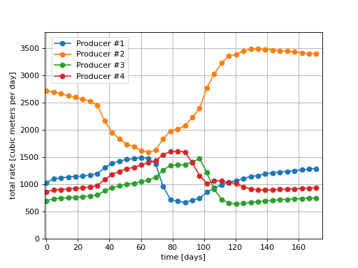
We have instructed GEOS to output the time series of rates for each producer. The data contained in the corresponding HDF5 files can be extracted and plotted as shown below.
To go further
Feedback on this example
This concludes the example on setting up a Dead-Oil simulation in the Egg model. For any feedback on this example, please submit a GitHub issue on the project’s GitHub page.
For more details
A complete description of the reservoir flow solver is found here: Compositional Multiphase Flow Solver.
The well solver is description at Compositional Multiphase Well Solver.
The available constitutive models are listed at Constitutive Models.