Vertical PoroElasto-Plastic Wellbore Problem
Context
The main objective of this example is to demonstrate how to use the internal wellbore mesh generator and poromechanical solvers in GEOS to tackle wellbore problems in porous media. In this example, a poroplastic model is applied to find the solution of rock deformation within the vicinity of a vertical wellbore, considering elastoplastic deformation, fluid diffusion and poromechanical coupling effect. To do so, a single phase flow solver is fully coupled with a Lagrangian mechanics solver and the Extended Drucker-Prager model (see Model: Extended Drucker-Prager) is chosen as the material model for the solid domain. We first solve this problem with a poroelastic model and verify the modeling results with the corresponding analytical solutions. Then, the verified case is modified to test a poroplastic version, whose results are compared with the ones obtained from the poroelastic case to highlight the impact of plasticity in this specific problem.
Objectives
At the end of this example you will know:
how to construct meshes for wellbore problems with the internal wellbore mesh generator,
how to specify initial and boundary conditions, such as reservoir properties, in-situ stresses, mixed loading (mechanical and fluid) at wellbore wall and far-field constraints,
how to use multiple solvers in GEOS for predicting poroplastic deformations in the near wellbore region.
Input file
This example uses no external input files and everything required is contained within a single GEOS input file.
The xml input files for the test case with poroelasticity are located at:
inputFiles/poromechanics/PoroElasticWellbore_base.xml
inputFiles/poromechanics/PoroElasticWellbore_benchmark.xml
The xml input files for the test case with poroplasticity are located at:
inputFiles/poromechanics/PoroDruckerPragerWellbore_base.xml
inputFiles/poromechanics/PoroDruckerPragerWellbore_benchmark.xml
Description of the case
We simulate the wellbore problem subjected to anisotropic horizontal stress ( and
and  ) and vertical stress (
 ), as shown below. This is a vertical wellbore, which is drilled in a porous medium. By changing the wellbore supporting pressure, the mechanical deformation of the reservoir rock will be induced and evolve with time, due to fluid diffusion and coupling effect. Considering inelastic constitutive behavior, the reservoir rock in the near wellbore region will experience elastoplastic deformation and a plastic zone will be developed and expand with time. To setup the base case, a poroelastic version is employed to find the poroelastic solutions of this wellbore problem, which are verified with the analytical solution (Detournay and Cheng, 1993) from the literature. Following that, a poroplastic version is built and used to obtain the temporal and spatial solutions of pore pressure, displacement and stress fields around the wellbore, considering induced plastic deformation.
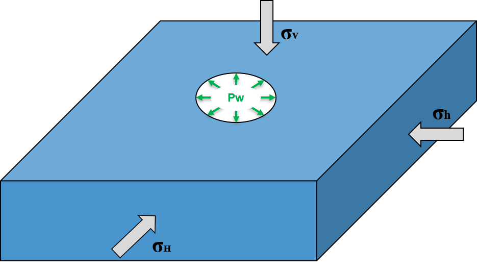
Fig. 52 Sketch of the wellbore problem
All inputs for this case are contained inside a single XML file.
In this example, we focus our attention on the Mesh tags, the Solver tags, the Constitutive tags, and the FieldSpecifications tags.
Mesh
The following figure shows the generated mesh that is used for solving this wellbore problem
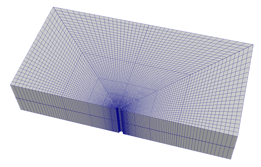
Fig. 53 Generated mesh for the wellbore problem
Let us take a closer look at the geometry of this wellbore problem.
We use the internal mesh generator InternalWellbore to create a rock domain
( ), with a wellbore of
initial radius equal to
), with a wellbore of
initial radius equal to  m.
Coordinates of
m.
Coordinates of trajectory defines the wellbore trajectory, which represents a perfect vertical well in this example.
By turning on autoSpaceRadialElems="{ 1 }", the internal mesh generator automatically sets number and spacing of elements in the radial direction, which overrides the values of nr.
With useCartesianOuterBoundary="0", a Cartesian aligned outer boundary on the outer block is enforced.
In this way, a structured three-dimensional mesh is created with 100 x 80 x 2 elements in the radial, tangential and z directions, respectively. All the elements are eight-node hexahedral elements (C3D8) and refinement is performed
to conform with the wellbore geometry. This mesh is defined as a cell block with the name
cb1.
<Mesh>
  <InternalWellbore
    name="mesh1"
    elementTypes="{ C3D8 }"
    radius="{ 0.1, 5.0 }"
    theta="{ 0, 180 }"
    zCoords="{ -1, 1 }"
    nr="{ 40 }"
    nt="{ 80 }"
    nz="{ 2 }"
    trajectory="{ { 0.0, 0.0, -1.0 },
                  { 0.0, 0.0,  1.0 } }"
    autoSpaceRadialElems="{ 1 }"
    useCartesianOuterBoundary="0"
    cellBlockNames="{ cb1 }"/>
</Mesh>
Solid mechanics solver
GEOS is a multi-physics platform. Different combinations of
physics solvers available in the code can be applied
in different regions of the domain and be functional at different stages of the simulation.
The Solvers tag in the XML file is used to list and parameterize these solvers.
To specify a coupling between two different solvers, we define and characterize each single-physics solver separately. Then, we customize a coupling solver between these single-physics solvers as an additional solver. This approach allows for generality and flexibility in constructing multi-physics solvers. The order of specifying these solvers is not restricted in GEOS. Note that end-users should give each single-physics solver a meaningful and distinct name, as GEOS will recognize these single-physics solvers based on their customized names and create user-expected coupling.
As demonstrated in this example, to setup a poromechanical coupling, we need to define three different solvers in the XML file:
the mechanics solver, a solver of type
SolidMechanicsLagrangianFEMcalled heremechanicsSolver(more information here: Solid Mechanics Solver),
<SolidMechanicsLagrangianFEM
  name="mechanicsSolver"
  logLevel="1"
  discretization="FE1"
  targetRegions="{ Omega }"
  >
  <NonlinearSolverParameters
    newtonTol = "1.0e-5"
    newtonMaxIter = "15"
  />
</SolidMechanicsLagrangianFEM>
the single-phase flow solver, a solver of type
SinglePhaseFVMcalled hereSinglePhaseFlowSolver(more information on these solvers at Singlephase Flow Solver),
<SinglePhaseFVM
  name="SinglePhaseFlowSolver"
  logLevel="1"
  discretization="singlePhaseTPFA"
  targetRegions="{Omega}">
  <NonlinearSolverParameters
    newtonTol = "1.0e-6"
    newtonMaxIter = "8"
  />
</SinglePhaseFVM>
</Solvers>
the coupling solver (
SinglePhasePoromechanics) that will bind the two single-physics solvers above, which is named asPoromechanicsSolver(more information at Poromechanics Solver).
<Solvers gravityVector="{0.0, 0.0, 0.0}">
<SinglePhasePoromechanics
  name="PoromechanicsSolver"
  solidSolverName="mechanicsSolver"
  flowSolverName="SinglePhaseFlowSolver"
  logLevel="1"
  targetRegions="{Omega}">
  <LinearSolverParameters
    solverType="direct"
    directParallel="0"
    logLevel="0"
  />
  <NonlinearSolverParameters
    newtonMaxIter = "40"
  />
</SinglePhasePoromechanics>
The two single-physics solvers are parameterized as explained in their corresponding documents.
In this example, let us focus on the coupling solver.
This solver (PoromechanicsSolver) uses a set of attributes that specifically describe the coupling process within a poromechanical framework.
For instance, we must point this solver to the designated fluid solver (here: SinglePhaseFlowSolver) and solid solver (here: mechanicsSolver).
These solvers are forced to interact through the porousMaterialNames="{porousRock}" with all the constitutive models. We specify the discretization method (FE1, defined in the NumericalMethods section), and the target regions (here, we only have one, Omega).
More parameters are required to characterize a coupling procedure (more information at Poromechanics Solver). In this way, the two single-physics solvers will be simultaneously called and executed for solving the wellbore problem here.
Discretization methods for multiphysics solvers
Numerical methods in multiphysics settings are similar to single physics numerical methods. In this problem, we use finite volume for flow and finite elements for solid mechanics. All necessary parameters for these methods are defined in the NumericalMethods section.
As mentioned before, the coupling solver and the solid mechanics solver require the specification of a discretization method called FE1.
In GEOS, this discretization method represents a finite element method
using linear basis functions and Gaussian quadrature rules.
For more information on defining finite elements numerical schemes,
please see the dedicated Finite Element Discretization section.
The finite volume method requires the specification of a discretization scheme.
Here, we use a two-point flux approximation scheme (singlePhaseTPFA), as described in the dedicated documentation (found here: Finite Volume Discretization).
<NumericalMethods>
  <FiniteElements>
    <FiniteElementSpace
      name="FE1"
      order="1"/>
    </FiniteElements>
  <FiniteVolume>
    <TwoPointFluxApproximation
      name="singlePhaseTPFA"
    />
  </FiniteVolume>
</NumericalMethods>
Constitutive laws
For this test problem, the solid and fluid materials are named as rock and water respectively, whose mechanical properties are specified in the Constitutive section. In this example, different material models, linear elastic isotropic model (see Model: Elastic Isotropic) and Extended Drucker-Prager model (see Model: Extended Drucker-Prager), are used to solve the mechanical deformation, which is the only difference between the poroelastic and poroplastic cases in this example.
For the poroelastic case, PorousElasticIsotropic model is used to describe the linear elastic isotropic response of rock to loading. And the single-phase fluid model CompressibleSinglePhaseFluid is selected to simulate the flow of water upon injection:
<Constitutive>
  <PorousElasticIsotropic
    name="porousRock"
    solidModelName="rock"
    porosityModelName="rockPorosity"
    permeabilityModelName="rockPerm"
  />
  <ElasticIsotropic
    name="rock"
    defaultDensity="2700"
    defaultBulkModulus="1.1111e10"
    defaultShearModulus="8.3333e9"
  />
  <CompressibleSinglePhaseFluid
    name="water"
    defaultDensity="1000"
    defaultViscosity="0.001"
    referencePressure="0e6"
    referenceDensity="1000"
    compressibility="2.09028227021e-10"
    referenceViscosity="0.001"
    viscosibility="0.0"
  />
  <BiotPorosity
    name="rockPorosity"
    defaultGrainBulkModulus="1.0e27"
    defaultReferencePorosity="0.3"
  />
  <ConstantPermeability
    name="rockPerm"
    permeabilityComponents="{1.0e-20, 1.0e-20, 1.0e-20}"
  />
</Constitutive>
For the poroplastic case, PorousExtendedDruckerPrager model is used to simulate the elastoplastic behavior of rock. And the single-phase fluid model CompressibleSinglePhaseFluid is employed to handle the storage and flow of water:
<Constitutive>
  <PorousExtendedDruckerPrager
    name="porousRock"
    solidModelName="rock"
    porosityModelName="rockPorosity"
    permeabilityModelName="rockPerm"
  />
  <ExtendedDruckerPrager
    name="rock"
    defaultDensity="2700"
    defaultBulkModulus="1.1111e10"
    defaultShearModulus="8.3333e9"
    defaultCohesion="1.0e6"
    defaultInitialFrictionAngle="15.27"
    defaultResidualFrictionAngle="23.05"
    defaultDilationRatio="1.0"
    defaultHardening="0.01"
  />
  <CompressibleSinglePhaseFluid
    name="water"
    defaultDensity="1000"
    defaultViscosity="0.001"
    referencePressure="0e6"
    referenceDensity="1000"
    compressibility="2.09028227021e-10"
    referenceViscosity="0.001"
    viscosibility="0.0"
  />
  <BiotPorosity
    name="rockPorosity"
    defaultGrainBulkModulus="1.0e27"
    defaultReferencePorosity="0.3"
  />
  <ConstantPermeability
    name="rockPerm"
    permeabilityComponents="{1.0e-20, 1.0e-20, 1.0e-20}"
  />
</Constitutive>
As for the material parameters, defaultInitialFrictionAngle, defaultResidualFrictionAngle and defaultCohesion denote the initial friction angle, the residual friction angle, and cohesion, respectively, as defined by the Mohr-Coulomb failure envelope.
As the residual friction angle defaultResidualFrictionAngle is larger than the initial one defaultInitialFrictionAngle, a strain hardening model is automatically chosen, whose hardening rate is given as defaultHardening="0.01".
If the residual friction angle is set to be less than the initial one, strain weakening will take place.
defaultDilationRatio="1.0" corresponds to an associated flow rule.
If using an incompressible fluid, the user can lower the fluid compressibility compressibility to 0.
The constitutive parameters such as the density, the bulk modulus, and the shear modulus are specified in the International System of Units. A stress-dependent porosity model rockPorosity and constant permeability rockPerm model are defined in this section.
Initial and boundary conditions
The next step is to specify fields, including:
The initial value (the in-situ stresses and pore pressure have to be initialized)
The boundary conditions (traction and fluid loading at the wellbore wall and constraints of the outer boundaries have to be set)
In this example, we need to specify anisotropic horizontal stress ( = -9.0 MPa and = -11.0 MPa) and vertical stress ( = -12.0 MPa).
A compressive traction (InnerMechanicalLoad)  = -10 MPa and fluid loading (
InnerFluidLoad)  = 10 MPa are applied at the wellbore wall
 rneg.
The remaining parts of the outer boundaries are subjected to roller constraints.
These boundary conditions are set up through the FieldSpecifications section.
<FieldSpecifications>
  <FieldSpecification
    name="stressXX"
    initialCondition="1"
    setNames="{all}"
    objectPath="ElementRegions/Omega/cb1"
    fieldName="rock_stress"
    component="0"
    scale="-9.0e6"
  />

  <FieldSpecification
    name="stressYY"
    initialCondition="1"
    setNames="{all}"
    objectPath="ElementRegions/Omega/cb1"
    fieldName="rock_stress"
    component="1"
    scale="-11.0e6"
  />

  <FieldSpecification
    name="stressZZ"
    initialCondition="1"
    setNames="{all}"
    objectPath="ElementRegions/Omega/cb1"
    fieldName="rock_stress"
    component="2"
    scale="-12.0e6"
  />

  <FieldSpecification
    name="initialPressure"
    initialCondition="1"
    setNames="{all}"
    objectPath="ElementRegions/Omega/cb1"
    fieldName="pressure"
    scale="0e6"
  />

  <FieldSpecification
    name="xconstraint"
    objectPath="nodeManager"
    fieldName="totalDisplacement"
    component="0"
    scale="0.0"
    setNames="{xneg, xpos}"
  />

  <FieldSpecification
    name="yconstraint"
    objectPath="nodeManager"
    fieldName="totalDisplacement"
    component="1"
    scale="0.0"
    setNames="{tneg, tpos, ypos}"
  />

  <FieldSpecification
    name="zconstraint"
    objectPath="nodeManager"
    fieldName="totalDisplacement"
    component="2"
    scale="0.0"
    setNames="{zneg, zpos}"
  />

  <Traction
    name="InnerMechanicalLoad"
    setNames="{ rneg }"
    objectPath="faceManager"
    scale="-10.0e6"
    tractionType="normal"
    functionName="timeFunction"
  />

  <FieldSpecification
    name="InnerFluidLoad"
    setNames="{ rneg }"
    objectPath="faceManager"
    fieldName="pressure"
    scale="10e6"
    functionName="timeFunction"
  />
</FieldSpecifications>
With tractionType="normal", traction is applied to the wellbore wall rneg as a pressure specified from the product of scale scale="-10.0e6" and the outward face normal.
A table function timeFunction is used to define the time-dependent loading.
The coordinates and values form a time-magnitude
pair for the loading time history. In this case, the loading magnitude is given as:
<Functions>
  <TableFunction
    name="timeFunction"
    inputVarNames="{time}"
    coordinates="{0.0, 0.1, 1e6}"
    values="{0.0, 1.0, 1.0}"
  />
</Functions>
You may note :
All initial value fields must have
initialConditionfield set to1;The
setNamefield points to the previously defined box to apply the fields;
nodeManagerandfaceManagerin theobjectPathindicate that the boundary conditions are applied to the element nodes and faces, respectively;
fieldNameis the name of the field registered in GEOS;Component
0,1, and2refer to the x, y, and z direction, respectively;And the non-zero values given by
scaleindicate the magnitude of the loading;Some shorthands, such as
xnegandxpos, are used as the locations where the boundary conditions are applied in the computational domain. For instance,xnegmeans the portion of the computational domain located at the left-most in the x-axis, whilexposrefers to the portion located at the right-most area in the x-axis. Similar shorthands includeypos,yneg,zpos, andzneg;The mud pressure loading has a negative value due to the negative sign convention for compressive stress in GEOS.
The parameters used in the simulation are summarized in the following table, which are specified in the
Constitutive and FieldSpecifications sections.
Symbol |
Parameter |
Unit |
Value |
|---|---|---|---|
|
Bulk Modulus |
[GPa] |
11.11 |
|
Shear Modulus |
[GPa] |
8.33 |
|
Cohesion |
[MPa] |
1.0 |
|
Initial Friction Angle |
[degree] |
15.27 |
|
Residual Friction Angle |
[degree] |
23.05 |
|
Hardening Rate |
[-] |
0.01 |
|
Min Horizontal Stress |
[MPa] |
-9.0 |
|
Max Horizontal Stress |
[MPa] |
-11.0 |
|
Vertical Stress |
[MPa] |
-12.0 |
|
Initial Well Radius |
[m] |
0.1 |
|
Traction at Well |
[MPa] |
-10.0 |
|
Fluid Pressure at Well |
[MPa] |
10.0 |
|
Fluid Density |
[kg/m3] |
1000.0 |
|
Fluid Viscosity |
[Pa s] |
0.001 |
|
Fluid Compressibility |
[Pa-1] |
2.09*10-10 |
|
Matrix Permeability |
[m2] |
1.0*10-20 |
|
Porosity |
[-] |
0.3 |


Inspecting results
As defined in the Events section, we run this simulation for 497640 seconds. In the above examples, we requested silo-format output files. We can therefore import these into VisIt and use python scripts to visualize the outcome. Please note that a non-dimensional time is used in the analytical solution, and the end time here leads to a non-dimensional end time of t* = 4.62.
Using the poroelastic solver, below figure shows the prediction of pore pressure distribution upon fluid injection.
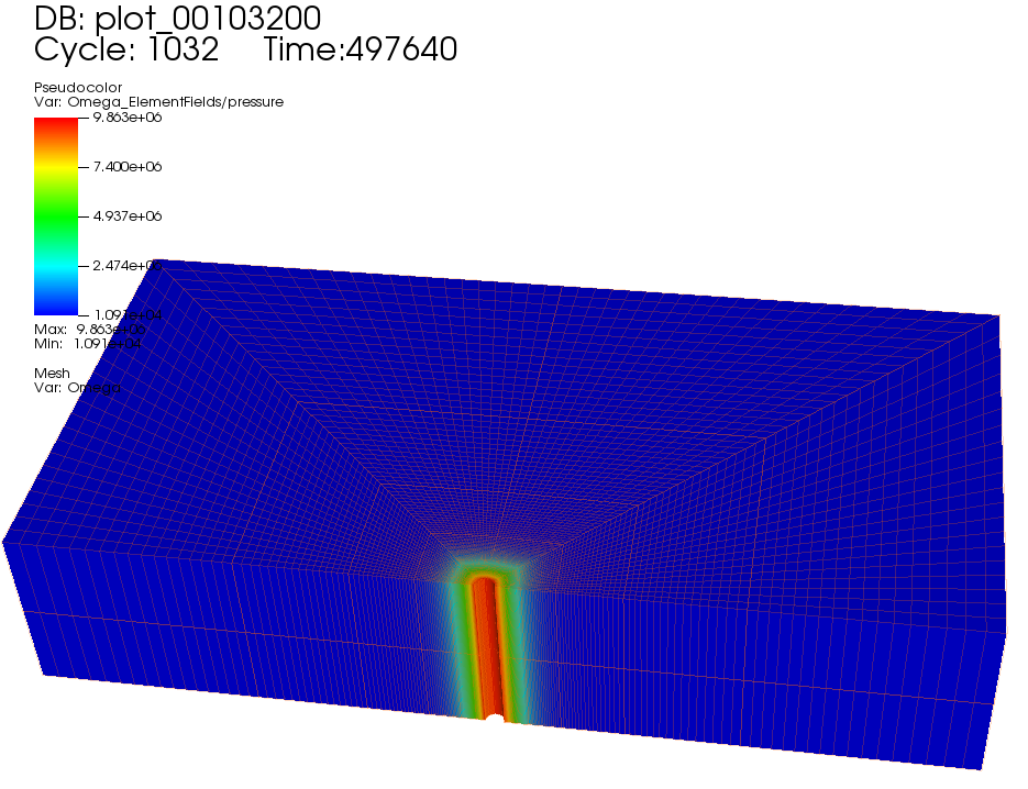
Fig. 54 Simulation result of pore pressure distribution
For the above poroelastic example, an analytical solution (Detournay and Cheng, 1993) is hereby employed to verify the accuracy of the numerical results. Following figure shows the comparisons between the numerical predictions (marks) and the corresponding analytical solutions (solid curves) with respect to the distributions of pore pressure, radial displacement, effective radial and tangential stresses along the minimum horizontal stress direction (x-axis). One can observe that GEOS results correlate very well with the analytical solutions for the poroelastic case.
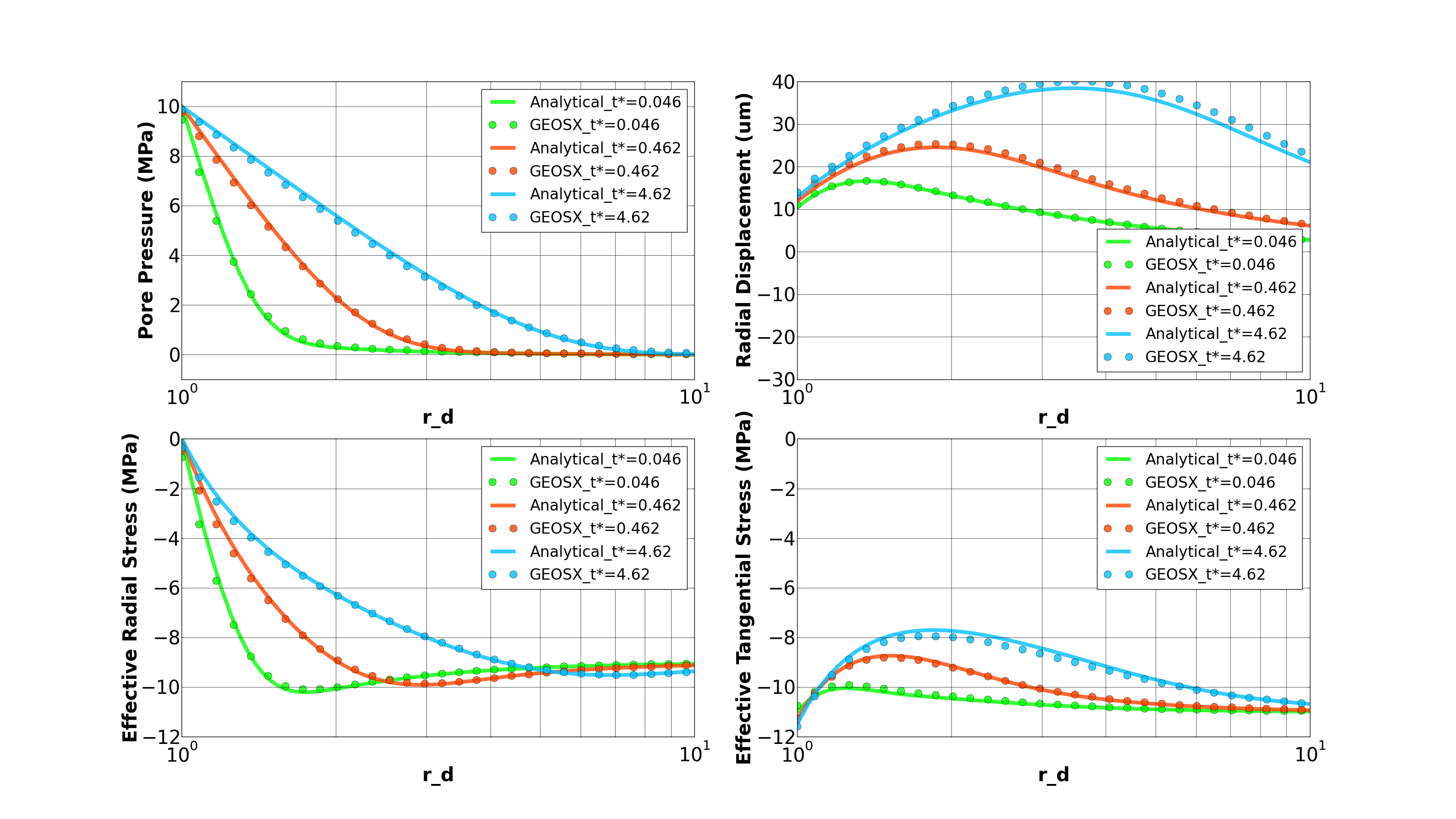
Fig. 55 Comparing GEOS results with analytical solutions
For the same 3D wellbore problem, the poroplastic case is thereafter tested and compared with the poroelastic one. The figure below shows the distribution of  in the near wellbore region for both cases. As expected, a relaxation of the tangential stress along the direction of minimum horizontal stress is detected, which can be attributed to the plastic response of the rock.
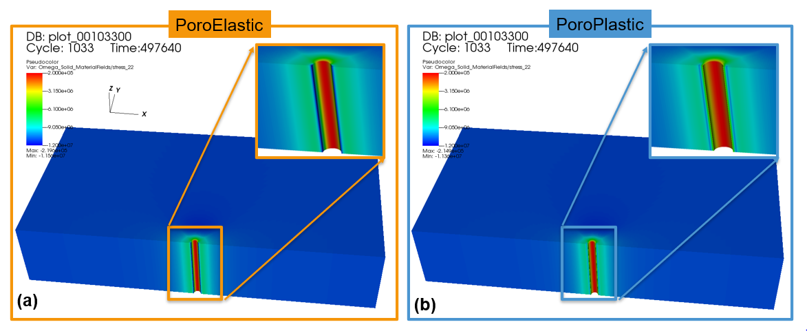
Fig. 56 Simulation result of Syy: PoroElastic vs. PoroPlastic
By using python scripts, we can extract the simulation results along any direction and provide detailed comparisons between different cases. Here, the pore pressure, radial displacement, radial and tangential effective stresses along the direction of minimum horizontal stress are obtained at different time steps and plotted against the corresponding ones of the poroelastic case. Because of fluid diffusion and coupling effect, following figure shows that these solutions evolve with time for both cases. As mentioned above, a plastic zone is developed in the vicinity of the wellbore, due to stress concentration. As for the far field region, these two cases become almost identical, with the rock deformation governed by poroelasticity.
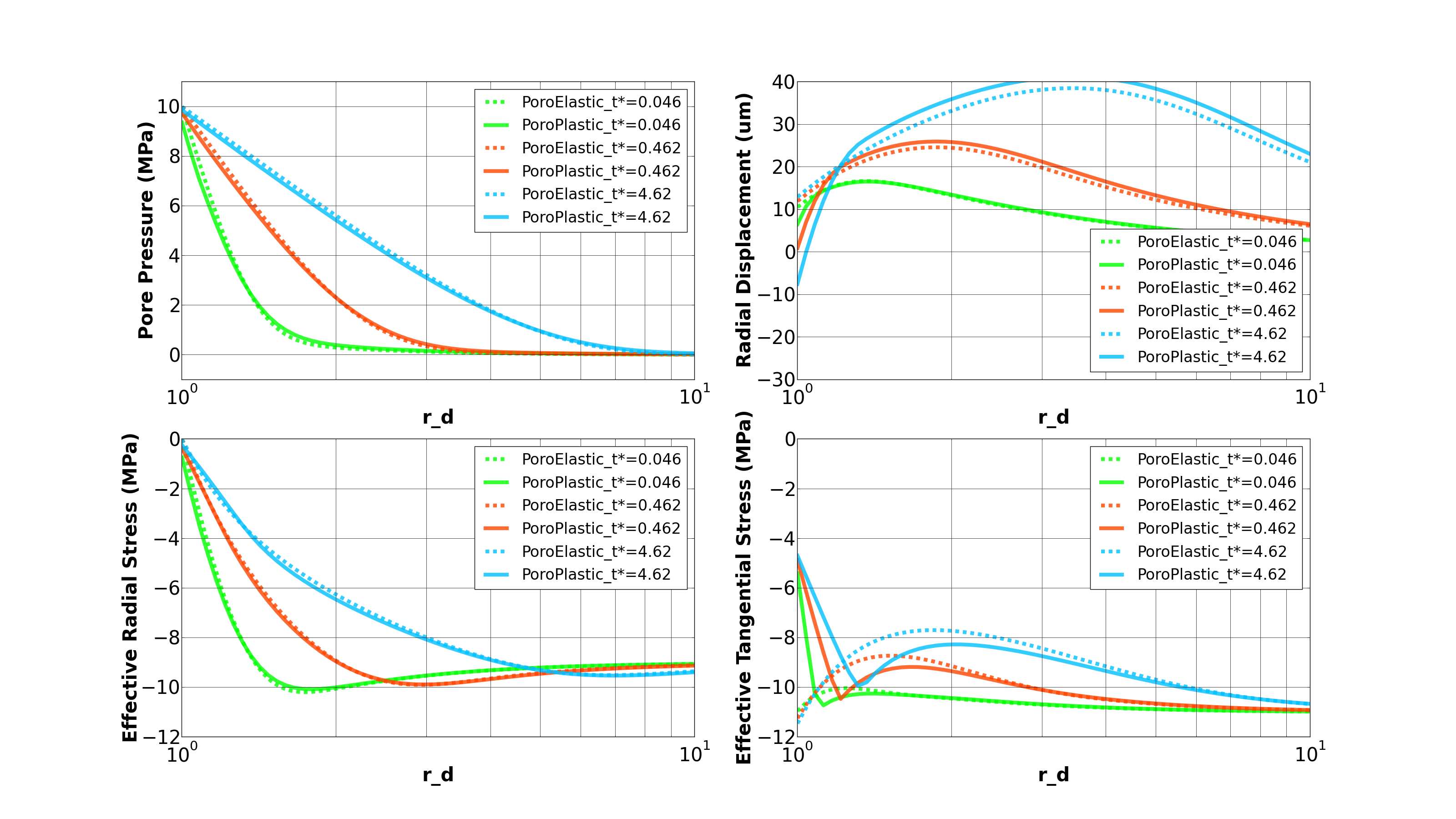
Fig. 57 Comparing the PoroPlastic case with the PoroElastic case at different times
To go further
Feedback on this example
This concludes the example on PoroPlasticity Model for Wellbore Problems. For any feedback on this example, please submit a GitHub issue on the project’s GitHub page.
For more details
More on plasticity models, please see Model: Extended Drucker-Prager.
More on multiphysics solvers, please see Poromechanics Solver.