Kirsch Wellbore Problem
Context
In this example, we simulate a vertical elastic wellbore subjected to in-situ stress and the induced elastic deformation of the reservoir rock. Kirsch’s solution to this problem provides the stress and displacement fields developing around a circular cavity, which is hereby employed to verify the accuracy of the numerical results. For this example, the TimeHistory function and python scripts are used to output and post-process multi-dimensional data (stress and displacement).
Input file
Everything required is contained within two GEOS input files located at:
inputFiles/solidMechanics/KirschProblem_base.xml
inputFiles/solidMechanics/KirschProblem_benchmark.xml
Description of the case
We solve a drained wellbore problem subjected to anisotropic horizontal stress ( and
and  ) as shown below. This is a vertical wellbore drilled in an infinite, homogeneous, isotropic, and elastic medium. Far-field in-situ stresses and internal supporting pressure acting at the circular cavity cause a mechanical deformation of the reservoir rock and stress concentration in the near-wellbore region. For verification purpose, a plane strain condition is considered for the numerical model.
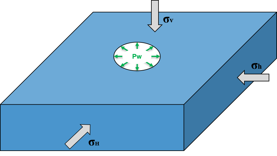
Fig. 42 Sketch of the wellbore problem
In this example, stress ( ,
,  , and
, and  ) and displacement (
 and
and  ) fields around the wellbore are calculated numerically. These numerical predictions are compared with the corresponding Kirsch solutions (Poulos and Davis, 1974).
![\sigma_{rr} = \frac{ \sigma_{xx} + \sigma_{yy} }{ 2 } {[ 1 - ( \frac{ a_0 }{ r })^{ 2 } ]} + \frac{ \sigma_{xx} - \sigma_{yy} }{ 2 } {[ 1 - 4 ( \frac{ a_0 }{ r })^{ 2 } + 3 ( \frac{ a_0 }{ r })^{ 4 } ]} \text{cos} \left( {2 \theta} \right) + P_w {( \frac{ a_0 }{ r })^{ 2 }}](../../../../../../_images/math/aba537c7b4dd1970e33d764ef0270ec25f22292a.svg)
![\sigma_{\theta\theta} = \frac{ \sigma_{xx} + \sigma_{yy} }{ 2 } {[ 1 + ( \frac{ a_0 }{ r })^{ 2 } ]} - \frac{ \sigma_{xx} - \sigma_{yy} }{ 2 } {[ 1 + 3 ( \frac{ a_0 }{ r })^{ 4 } ]} \text{cos} \left( {2 \theta} \right) - P_w {( \frac{ a_0 }{ r })^{ 2 }}](../../../../../../_images/math/79951e31c3ab7cb3e914e03e16125cb6121d80f8.svg)
![\sigma_{r\theta} = - \frac{ \sigma_{xx} - \sigma_{yy} }{ 2 } {[ 1 + 2 ( \frac{ a_0 }{ r })^{ 2 } - 3 ( \frac{ a_0 }{ r })^{ 4 } ]} \text{sin} \left( {2 \theta} \right)](../../../../../../_images/math/75fe6f9a51ef755d72b6d3c606cd5c2c9ab03bf8.svg)
![u_{r} = - \frac{ ( a_0 )^{ 2 } }{ 2Gr } {[ \frac{ \sigma_{xx} + \sigma_{yy} }{ 2 } + \frac{ \sigma_{xx} - \sigma_{yy} }{ 2 } {( 4 ( 1- \nu ) - ( \frac{ a_0 }{ r })^{ 2 } )} \text{cos} \left( {2 \theta} \right) - P_w ]}](../../../../../../_images/math/fc8cf09ec06dea3d2b9ee18e55275c8c381a9050.svg)
![u_{\theta} = \frac{ ( a_0 )^{ 2 } }{ 2Gr } { \frac{ \sigma_{xx} - \sigma_{yy} }{ 2 } {[ 2 (1- 2 \nu) + ( \frac{ a_0 }{ r })^{ 2 } ]} \text{sin} \left( {2 \theta} \right) }](../../../../../../_images/math/d504de60a4414f26ab1555c7128edd3713cb1ceb.svg)
where  is the intiial wellbore radius,
  is the radial coordinate,
  is the Poisson’s ratio,
  is the shear modulus,
  is the normal traction acting on the wellbore wall, the angle
  is measured with respect to x-z plane and defined as positive in counter-clockwise direction.
In this example, we focus our attention on the Mesh,
the Constitutive, and the FieldSpecifications tags.
Mesh
Following figure shows the generated mesh that is used for solving this wellbore problem.
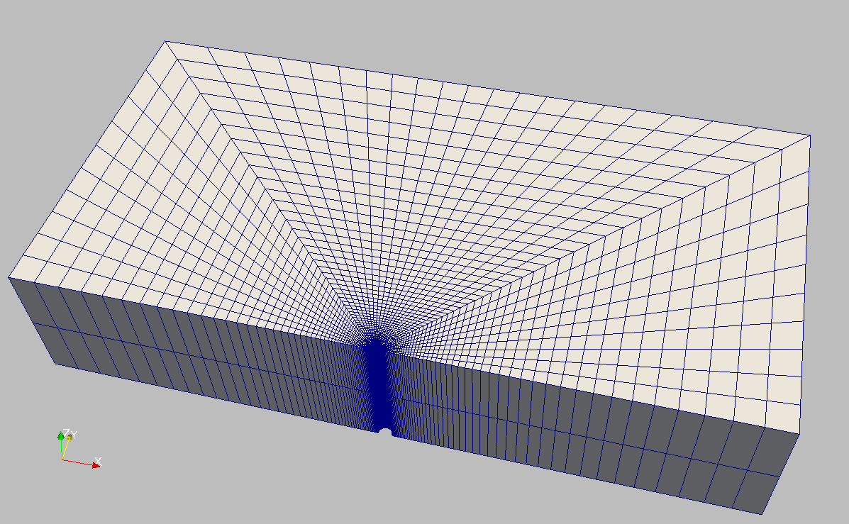
Fig. 43 Generated mesh for a vertical wellbore problem
Let us take a closer look at the geometry of this wellbore problem.
We use the internal wellbore mesh generator InternalWellbore to create a rock domain
( ), with a wellbore of
initial radius equal to
), with a wellbore of
initial radius equal to  m.
Only half of the domain is modeled by a
m.
Only half of the domain is modeled by a theta angle from 0 to 180, assuming symmetry for the rest of the domain.
Coordinates of trajectory defines the wellbore trajectory, a vertical well in this example.
By turning on autoSpaceRadialElems="{ 1 }", the internal mesh generator automatically sets number and spacing of elements in the radial direction, which overrides the values of nr.
With useCartesianOuterBoundary="0", a Cartesian aligned boundary condition is enforced on the outer blocks.
This way, a structured three-dimensional mesh is created with 50 x 40 x 2 elements in the radial, tangential and z directions, respectively. All elements are eight-node hexahedral elements (C3D8) and refinement is performed
to conform with the wellbore geometry. This mesh is defined as a cell block with the name
cb1.
  <Mesh>
    <InternalWellbore
      name="mesh1"
      elementTypes="{ C3D8 }"
      radius="{ 0.1, 5.0 }"
      theta="{ 0, 180 }"
      zCoords="{ -1, 1 }"
      nr="{ 40 }"
      nt="{ 40 }"
      nz="{ 2 }"
      trajectory="{ { 0.0, 0.0, -1.0 },
                    { 0.0, 0.0, 1.0 } }"
      autoSpaceRadialElems="{ 1 }"
      useCartesianOuterBoundary="0"
      cellBlockNames="{ cb1 }"/>
  </Mesh>
Solid mechanics solver
For a drained wellbore problem, the pore pressure variation is omitted. Therefore, we just need to define a solid mechanics solver, which is called mechanicsSolver.
This solid mechanics solver (see Solid Mechanics Solver) is based on the Lagrangian finite element formulation.
The problem is run as QuasiStatic without considering inertial effects.
The computational domain is discretized by FE1, which is defined in the NumericalMethods section.
The material is named rock, whose mechanical properties are specified in the Constitutive section.
  <Solvers gravityVector="{0.0, 0.0, 0.0}">
    <SolidMechanicsLagrangianFEM
      name="mechanicsSolver"
      logLevel="1"
      discretization="FE1"
      targetRegions="{Omega}">
      <NonlinearSolverParameters
        newtonTol = "1.0e-5"
        newtonMaxIter = "15"
      />
      <LinearSolverParameters
        directParallel="0"/>
    </SolidMechanicsLagrangianFEM>
  </Solvers>
Constitutive laws
For this drained wellbore problem, we simulate a linear elastic deformation around the circular cavity.
A homogeneous and isotropic domain with one solid material is assumed, with mechanical properties specified in the Constitutive section:
  <Constitutive>
    <ElasticIsotropic
      name="rock"
      defaultDensity="2700"
      defaultBulkModulus="5.0e8"
      defaultShearModulus="3.0e8"
    />
  </Constitutive>
Recall that in the SolidMechanicsLagrangianFEM section,
rock is the material in the computational domain.
Here, the isotropic elastic model ElasticIsotropic simulates the mechanical behavior of rock.
The constitutive parameters such as the density, the bulk modulus, and the shear modulus are specified in the International System of Units.
Time history function
In the Tasks section, PackCollection tasks are defined to collect time history information from fields.
Either the entire field or specified named sets of indices in the field can be collected.
In this example, stressCollection and displacementCollection tasks are specified to output the resultant stresses (tensor stored as an array with Voigt notation) and total displacement field (stored as a 3-component vector) respectively.
Note: The output field named averageStress (comprising six components per cell) represents the cell-wise average of each stress component, calculated using the finite element quadrature rule. The same definition applies to averageStrain.
  <Tasks>
    <PackCollection
      name="stressCollection"
      objectPath="ElementRegions/Omega/cb1"
      fieldName="averageStress"/>

    <PackCollection
      name="displacementCollection"
      objectPath="nodeManager"
      fieldName="totalDisplacement"/>
  </Tasks>
These two tasks are triggered using the Event management, where PeriodicEvent are defined for these recurring tasks.
GEOS writes two files named after the string defined in the filename keyword and formatted as HDF5 files (displacement_history.hdf5 and stress_history.hdf5). The TimeHistory file contains the collected time history information from each specified time history collector. This information includes datasets for the simulation time, element center or nodal position, and the time history information. Then, a Python script is prepared to access and plot any specified subset of the time history data for verification and visualization.
Initial and boundary conditions
The next step is to specify fields, including:
The initial value (the in-situ stresses and traction at the wellbore wall have to be initialized),
The boundary conditions (constraints of the outer boundaries have to be set).
Here, we specify anisotropic horizontal stress values ( = -9.0 MPa and = -11.25 MPa) and a vertical stress ( = -15.0 MPa).
A compressive traction (
= -15.0 MPa).
A compressive traction (WellLoad) = -2.0 MPa is loaded at the wellbore wall rneg.
The remaining parts of the outer boundaries are subjected to roller constraints.
These boundary conditions are set in the FieldSpecifications section.
  <FieldSpecifications>
    <FieldSpecification
      name="Sxx"
      initialCondition="1"
      setNames="{ all }"
      objectPath="ElementRegions"
      fieldName="rock_stress"
      component="0"
      scale="-11.25e6"
    />

    <FieldSpecification
      name="Syy"
      initialCondition="1"
      setNames="{ all }"
      objectPath="ElementRegions"
      fieldName="rock_stress"
      component="1"
      scale="-9.0e6"
    />

    <FieldSpecification
      name="Szz"
      initialCondition="1"
      setNames="{ all }"
      objectPath="ElementRegions"
      fieldName="rock_stress"
      component="2"
      scale="-15.0e6"
    />

    <Traction
      name="WellLoad"
      setNames="{ rneg }"
      objectPath="faceManager"
      scale="-2.0e6"
      tractionType="normal"
    />

    <FieldSpecification
      name="xconstraint"
      objectPath="nodeManager"
      fieldName="totalDisplacement"
      component="0"
      scale="0.0"
      setNames="{xneg, xpos}"
    />

    <FieldSpecification
      name="yconstraint"
      objectPath="nodeManager"
      fieldName="totalDisplacement"
      component="1"
      scale="0.0"
      setNames="{tneg, tpos, ypos}"
    />

    <FieldSpecification
      name="zconstraint"
      objectPath="nodeManager"
      fieldName="totalDisplacement"
      component="2"
      scale="0.0"
      setNames="{zneg, zpos}"
    />
  </FieldSpecifications>
With tractionType="normal", traction is applied to the wellbore wall rneg as a pressure specified as the scalar product of scale scale="-2.0e6" and the outward face normal vector.
In this case, the loading magnitude of the traction does not change with time.
You may note :
All initial value fields must have
initialConditionfield set to1;The
setNamefield points to the previously defined set to apply the fields;
nodeManagerandfaceManagerin theobjectPathindicate that the boundary conditions are applied to the element nodes and faces, respectively;
fieldNameis the name of the field registered in GEOS;Component
0,1, and2refer to the x, y, and z direction, respectively;And the non-zero values given by
scaleindicate the magnitude of the loading;Some shorthand, such as
xnegandxpos, are used as the locations where the boundary conditions are applied in the computational domain. For instance,xnegmeans the face of the computational domain located at the left-most extent in the x-axis, whilexposrefers to the face located at the right-most extent in the x-axis. Similar shorthands includeypos,yneg,zpos, andzneg;The mud pressure loading and in situ stresses have negative values due to the negative sign convention for compressive stress in GEOS.
The parameters used in the simulation are summarized in the following table.
Symbol |
Parameter |
Unit |
Value |
|---|---|---|---|
|
Bulk Modulus |
[MPa] |
500.0 |
|
Shear Modulus |
[MPa] |
300.0 |
|
Min Horizontal Stress |
[MPa] |
-9.0 |
|
Max Horizontal Stress |
[MPa] |
-11.25 |
|
Vertical Stress |
[MPa] |
-15.0 |
|
Initial Well Radius |
[m] |
0.1 |
|
Traction at Well |
[MPa] |
-2.0 |

Inspecting results
In the above examples, we request VTK output files that can be imported into Paraview to visualize the outcome. The following figure shows the distribution of in the near wellbore region.
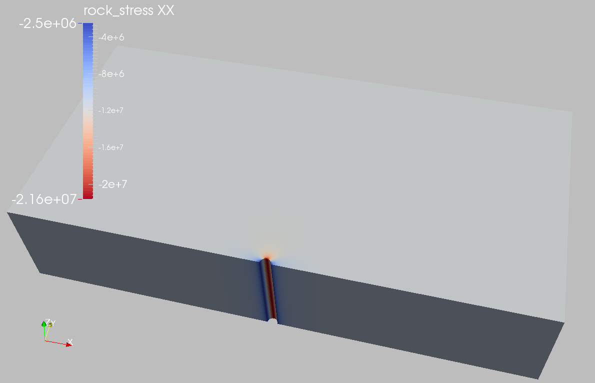
Fig. 44 Simulation result of
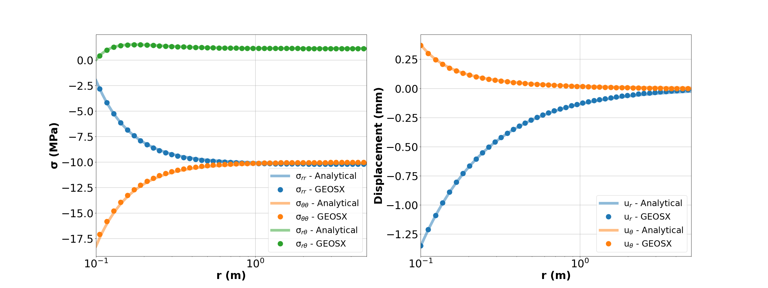
We use time history function to collect time history information and run a Python script to query and plot the results. The figure below shows the comparisons between the numerical predictions (marks) and the corresponding analytical solutions (solid curves) with respect to the distributions of stress components and displacement at = 45 degrees. Predictions computed by GEOS match the analytical results.
To go further
Feedback on this example
For any feedback on this example, please submit a GitHub issue on the project’s GitHub page.