CO2 Plume Evolution With Hysteresis Effect on Relative Permeability

Context

We consider a benchmark problem used in (Class et al., 2009) to compare a number of numerical models applied to CO2 storage in geological formations. Using a simplified miscible two-phase setup, this test case illustrates the modeling of solubility trapping (with CO2 dissolution in brine) and residual trapping (with gas relative permeability hysteresis) in CO2-brine systems.

Our goal is to review the different sections of the XML file reproducing the benchmark configuration and to demonstrate that the GEOS results (i.e., mass of CO2 dissolved and mobile for both hysteretic and non-hysteretic configurations) are in agreement with the reference results published in (Class et al., 2009) Problems 3.1 and 3.2.

Input file

This benchmark test is based on the XML file located below:

../../../../../../../inputFiles/compositionalMultiphaseWell/benchmarks/Class09Pb3/class09_pb3_smoke_3d.xml
../../../../../../../inputFiles/compositionalMultiphaseWell/benchmarks/Class09Pb3/class09_pb3_drainageOnly_iterative_base.xml

Problem description

The following text is adapted from the detailed description of the benchmark test case presented in (Class et al., 2009).

The setup is illustrated in the figure below. The mesh can be found in GEOSDATA and was provided for the benchmark. It discretizes the widely-used Johansen reservoir, which consists in a tilted reservoir with a main fault. The model domain has the following dimensions: 9600 x 8900 x [90-140] m. Both porosity and permeability are heterogeneous and given at vertices. A single CO2 injection well is located at (x,y) = (5440,3300) m with perforations only in the bottom 50 m of the reservoir. The injection takes place during the first 25 years of the 50-year simulation at the constant rate of 15 kg/s. A hydrostatic pressure gradient is imposed on the boundary faces as well as a constant geothermal gradient of 0.03 K/m.

The authors have used the following simplifying assumptions:

• The formation is isotropic.

• The temperature is constant in time.

• The pressure conditions at the lateral boundaries are constant over time, and equal to the initial hydrostatic condition.

Mesh and element regions

The proposed conforming discretization is fully hexahedral. A VTK filter PointToCell is used to map properties from vertices to cells, which by default builds a uniform average of values over the cell. The structured mesh is generated using some helpers python scripts from the formatted Point/Cells list provided. It is then imported using meshImport

  <Mesh>
    <InternalMesh
      name="mesh1"
      elementTypes="{ C3D8 }"
      xCoords="{ 5240, 5640 }"
      yCoords="{ 3100, 3500 }"
      zCoords="{ -3000, -2950 }"
      nx="{ 5 }"
      ny="{ 5 }"
      nz="{ 5 }"
      cellBlockNames="{ 1_hexahedra }">
      <InternalWell
        name="wellInjector1"
        wellRegionName="wellRegion"
        wellControlsName="wellControls"
        logLevel="1"
        polylineNodeCoords="{ { 5440.0, 3300.0, -2950.0 },
                              { 5440.0, 3300.0, -3000.00 } }"
        polylineSegmentConn="{ { 0, 1 } }"
        radius="0.1"
        numElementsPerSegment="5">
        <Perforation
          name="injector1_perf1"
          distanceFromHead="45"/>
        <Perforation
          name="injector1_perf2"
          distanceFromHead="35"/>
        <Perforation
          name="injector1_perf3"
          distanceFromHead="25"/>
        <Perforation
          name="injector1_perf4"
          distanceFromHead="15"/>
        <Perforation
          name="injector1_perf5"
          distanceFromHead="5"/>
      </InternalWell>
    </InternalMesh>
  </Mesh>

The central wellbore is discretized internally by GEOS (see CO 2 Injection). It includes five segments with a perforation in each segment. It has its own region wellRegion and control labeled wellControls defined and detailed respectively in ElementRegions and Solvers (see below). In the ElementRegions block,

  <ElementRegions>
    <CellElementRegion
      name="reservoir"
      cellBlocks="{ 1_hexahedra }"
      materialList="{ fluid, rock, relperm, cappres }"/>

    <WellElementRegion
      name="wellRegion"
      materialList="{ fluid, relperm, cappres }"/>
  </ElementRegions>

one single reservoir region labeled reservoir. A second region wellRegion is associated with the well. All those regions define materials to be specified inside the Constitutive block.

Coupled solver

The simulation is performed by the GEOS coupled solver for multiphase flow and well defined in the XML block CompositionalMultiphaseReservoir:

    <CompositionalMultiphaseFVM
      name="compositionalMultiphaseFlow"
      targetRegions="{ reservoir }"
      discretization="fluidTPFA"
      temperature="363"
      maxCompFractionChange="0.2"
      logLevel="1"
      useMass="1"/>

It references the two coupled solvers under the tags flowSolverName and wellSolverName. These are defined inside the same Solvers block following this coupled solver. It also defined non-linear, NonlinearSolverParameters and and linear, LinearSolverParameters, strategies.

The next two blocks are used to define our two coupled physics solvers compositionalMultiphaseFlow (of type CompositionalMultiphaseFVM) and compositionalMultiphaseWell (of type CompositionalMultiphaseWell).

Flow solver

We use the targetRegions attribute to define the regions where the flow solver is applied.

    <CompositionalMultiphaseReservoir
      name="coupledFlowAndWells"
      flowSolverName="compositionalMultiphaseFlow"
      wellSolverName="compositionalMultiphaseWell"
      logLevel="1"
      initialDt="1e2"
      targetRegions="{ reservoir, wellRegion }">
      <NonlinearSolverParameters
        newtonTol="1.0e-5"
        newtonMaxIter="40"/>
      <LinearSolverParameters
        solverType="fgmres"
        preconditionerType="mgr"
        krylovTol="1e-6"
        logLevel="1"/>
    </CompositionalMultiphaseReservoir>

The FV scheme discretization used is TPFA (which definition can be found nested in NumericalMethods/FiniteVolume) and some parameter values.

Well solver

The well solver is applied on its own region wellRegion which consists of the five discretized segments. It is also the place where the WellControls are set thanks to type, control, injectionStream , injectionTemperature, targetTotalRateTableName and, targetBHP for instance if we consider an injection well.

For more details on the wellbore modeling please refer to Compositional Multiphase Well Solver.

    <CompositionalMultiphaseWell
      name="compositionalMultiphaseWell"
      targetRegions="{ wellRegion }"
      logLevel="1"
      useMass="1">
      <WellControls
        name="wellControls"
        logLevel="1"
        type="injector"
        control="totalVolRate"
        referenceElevation="-3000"
        targetBHP="1e8"
        enableCrossflow="0"
        useSurfaceConditions="1"
        surfacePressure="101325"
        surfaceTemperature="288.71"
        targetTotalRateTableName="totalRateTable"
        injectionTemperature="353.15"
        injectionStream="{ 1.0, 0.0 }"/>
    </CompositionalMultiphaseWell>

Constitutive laws

This benchmark test involves a compositional mixture that defines two phases (CO2-rich and aqueous) labeled as gas and water which contain two components co2 and water. The miscibility of CO2 results in the presence of CO2 in the aqueous phase. The vaporization of H2O in the CO2-rich phase is not considered here.

    <CO2BrineEzrokhiFluid
      name="fluid"
      phaseNames="{ gas, water }"
      componentNames="{ co2, water }"
      componentMolarWeight="{ 44e-3, 18e-3 }"
      phasePVTParaFiles="{ tables/pvtgas.txt, tables/pvtliquid_ez.txt }"
      flashModelParaFile="tables/co2flash.txt"/>

The brine properties are modeled using Ezrokhi correlation, hence the block name CO2BrineEzrokhiFluid. The external PVT files tables/pvtgas.txt and tables/pvtliquid_ex.txt give access to the models considered respectively for the computation of gas density and viscosity and the brine density and viscosity, along with pressure, temperature, salinity discretization of the parameter space. The external file tables/co2flash.txt gives the same type of information for the CO2Solubility model (see CO2-brine model for details).

The rock model defines a slightly compressible porous medium with a reference porosity equal to 0.1.

    <CompressibleSolidConstantPermeability
      name="rock"
      solidModelName="nullSolid"
      porosityModelName="rockPorosity"
      permeabilityModelName="rockPerm"/>
    <NullModel
      name="nullSolid"/>
    <PressurePorosity
      name="rockPorosity"
      defaultReferencePorosity="0.1"
      referencePressure="1.0e7"
      compressibility="4.5e-10"/>
    <ConstantPermeability
      name="rockPerm"
      permeabilityComponents="{ 1.0e-12, 1.0e-12, 1.0e-12 }"/>

The relative permeability model is input through tables thanks to TableRelativePermeability block.

    <TableRelativePermeability
      name="relperm"
      phaseNames="{ gas, water }"
      wettingNonWettingRelPermTableNames="{ waterRelativePermeabilityTable,
                                            gasRelativePermeabilityTable }"/>

As this benchmark is testing the sensitivity of the plume dynamics to the relative permeability hysteresis modeling, in commented block the TableRelativePermeabilityHysteresis block sets up bounding curves for imbibition and drainage under imbibitionNonWettingRelPermTableName, imbibitionWettingRelPermTableName and, drainageWettingNonWettingRelPermTableNames compared to the wettingNonWettingRelPermTableNames label of the drainage only TableRelativePermeability blocks. Those link to TableFunction blocks in Functions, which define sample points for piecewise linear interpolation. This feature is used and explained in more details in the following section dedicated to Initial and Boundary conditions.

See,

../../../../../../../inputFiles/compositionalMultiphaseWell/benchmarks/Class09Pb3/class09_pb3_hystRelperm_iterative_base.xml

for the input base with relative permeability hysteresis setup.

    <TableRelativePermeabilityHysteresis
      name="relperm"
      phaseNames="{ gas, water }"
      drainageWettingNonWettingRelPermTableNames="{ drainageWaterRelativePermeabilityTable,
                                                  drainageGasRelativePermeabilityTable }"
      imbibitionNonWettingRelPermTableName="imbibitionGasRelativePermeabilityTable"      
      imbibitionWettingRelPermTableName="imbibitionWaterRelativePermeabilityTable"/>

Note

wettingNonWettingRelPermTableNames in TableRelativePermeability and drainageWettingNonWettingRelPermTableNames in TableRelativePermeabilityHysteresis are identical.

Capillary pressure is also tabulated and defined in TableCapillaryPressure. No hysteresis is modeled yet on the capillary pressure.

    <TableCapillaryPressure
      name="cappres"
      phaseNames="{ gas, water }"
      wettingNonWettingCapPressureTableName="waterCapillaryPressureTable"/>

Initial and boundary conditions

The domain is initially saturated with brine with a hydrostatic pressure field. This is specified using the HydrostaticEquilibrium XML tag in the FieldSpecifications block. The datum pressure and elevation used below are defined in (Class et al., 2009)).

   <HydrostaticEquilibrium
      name="equil"
      objectPath="ElementRegions"
      datumElevation="-3000"
      datumPressure="3.0e7"
      initialPhaseName="water"
      componentNames="{ co2, water }"
      componentFractionVsElevationTableNames="{ initCO2CompFracTable,
                                                initWaterCompFracTable }"
      temperatureVsElevationTableName="initTempTable"/>

In the Functions block, the TableFunction s named initCO2CompFracTable and initWaterCompFracTable define the brine-saturated initial state, while the TableFunction named initTempTable defines the temperature field as a function of depth to impose the geothermal gradient.

The boundaries are set to have a constant 0.03 K/m temperature gradient as well as the hydrostatic pressure gradient. We supplement that with water dominant content. Each block is linking a fieldName to a TableFunction tagged as the value of functionName. In order to have those imposed on the boundary faces, we provide faceManager as objectPath.

    <FieldSpecification
      name="bcPressure"
      objectPath="faceManager"
      setNames="{3}"
      fieldName="pressure"
      functionName="pressureFunction"
      scale="1"/>
    <FieldSpecification
      name="bcTemperature"
      objectPath="faceManager"
      setNames="{3}"
      fieldName="temperature"
      functionName="temperatureFunction"
      scale="1"/>
    <FieldSpecification
      name="bcCompositionCO2"
      objectPath="faceManager"
      setNames="{3}"
      fieldName="globalCompFraction"
      component="0"
      scale="0.000001"/>
    <FieldSpecification
      name="bcCompositionWater"
      objectPath="faceManager"
      setNames="{3}"
      fieldName="globalCompFraction"
      component="1"
      scale="0.999999"/>

Outputing reservoir statistics

In order to output partitioning of CO2 mass, we use reservoir statistics implemented in GEOS. This is done by defining a Task, with flowSolverName pointing to the dedicated solver and computeRegionStatistics set to 1 to compute statistics by regions. The setNames field is set to 3 as it is its attribute tag in the input vtu mesh.

    <CompositionalMultiphaseStatistics
      name="compflowStatistics"
      flowSolverName="compositionalMultiphaseFlow"
      logLevel="1"
      computeCFLNumbers="1"
      computeRegionStatistics="1"/>

and an Event for this to occur recursively with a forceDt argument for the period over which statistics are output and target pointing towards the aforementioned Task.

    <PeriodicEvent
      name="statistics"
      timeFrequency="1e5"
      target="/Tasks/compflowStatistics"/>

This is a sample of the output we will have in the log file.

compflowStatistics, reservoir: Pressure (min, average, max): 2.5139e+07, 2.93668e+07, 3.23145e+07 Pa
compflowStatistics, reservoir: Delta pressure (min, max): -12157, 158134 Pa
compflowStatistics, reservoir: Temperature (min, average, max): 293.15, 371.199, 379.828 K
compflowStatistics, reservoir: Total dynamic pore volume: 1.57994e+09 rm^3
compflowStatistics, reservoir: Phase dynamic pore volumes: { 1.00239e+06, 1.57894e+09 } rm^3
compflowStatistics, reservoir: Phase mass (including both trapped and non-trapped): { 7.24891e+08, 1.6245e+12 } kg
compflowStatistics, reservoir: Trapped phase mass: { 5.3075e+08, 3.2511e+11 } kg
compflowStatistics, reservoir: Dissolved component mass: { { 7.13794e+08, 4.53966e+06 }, { 1.6338e+08, 1.62433e+12 } } kg
compflowStatistics: Max phase CFL number: 65.1284
compflowStatistics: Max component CFL number: 2.32854

Note

The log file mentioned above could be an explicit printout of the stdio from MPI launch or the autogenerated output from a SLURM job slurm.out or similar

Inspecting results

We request VTK-format output files and use Paraview to visualize the results under the Outputs block.

The following figure shows the distribution of CO2 saturation thresholded above a significant value (here 0.001). The displayed cells are colored with respect to the CO2 mass they contain. If the relative permeability for the gas phase drops below 10e-7, the cell is displayed in black.

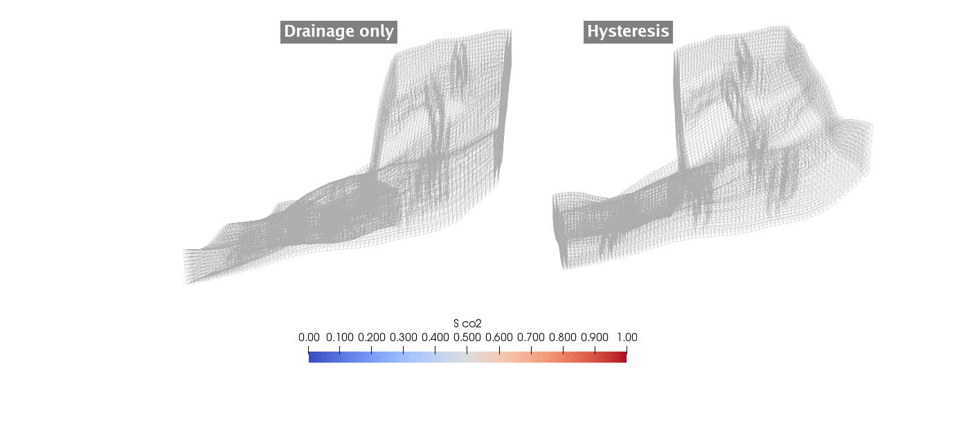
Fig. 13 Plume of CO2 saturation for significant value where immobile CO2 is colored in black.

We observe the importance of hysteresis modeling in CO2 plume migration. Indeed, during the migration phase, the cells at the tail of the plume are switching from drainage to imbibition and the residual CO2 is trapped. This results in a slower migration and expansion of the plume.

To validate the GEOS results, we consider the metrics used in (Class et al., 2009). The reporting values are the dissolved and gaseous CO2 with respect to time using only the drainage relative permeability and using hysteretic relative permeabilities.

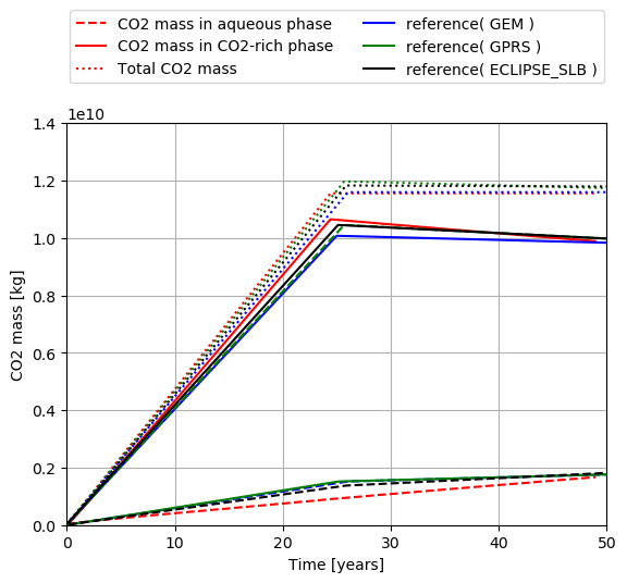
Fig. 14 CO2 mass in aqueous and CO2-rich phases as a function of without relative permeability hysteresis

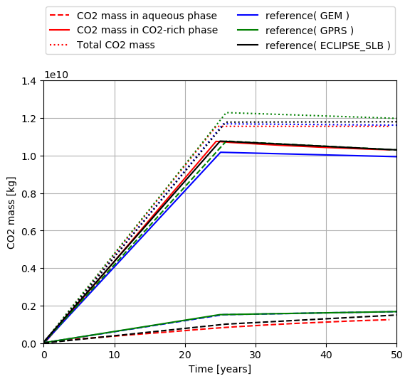
Fig. 15 CO2 mass in aqueous and CO2-rich phases as a function of time with relative permeability hysteresis

We can see that at the end of the injection period the mass of CO2 in the gaseous phase stops increasing and starts decreasing due to dissolution of CO2 in the brine phase. These curves confirm the agreement between GEOS and the results of (Class et al., 2009).

To go further

Feedback on this example

For any feedback on this example, please submit a GitHub issue on the project’s GitHub page.