Assessment of CO2 Storage residual and dissolution trapping mechanism
Context
We consider the benchmark proposed in (Nordbotten et al., 2024) to showcase the effect of the convective mixing in addition to the usually considered residual trapping in a multi-facies resevoir. Also, by using a thermal formulation, the effect of injecting cold CO2 can be observed.
This example can serve as a guideline to set-up the input XML deck to reproduce the published results on SPE11 CSP. The input decks for other simulators can be found at decks.
Note
We refer to the official comparative website to see all submitted results.
Brief case description
As the detailed description is available in (Nordbotten et al.,2024), we will only briefly review the data set that will be used to in the following sections and let the interested reader read the full version.
The spe11-b is a reservoir-like 2D case rescaled from the FluidFlower experiment. It consists in a 8.4 km large and 1.2 km deep reservoir which top depth is at 2km from the surface. A global geothermal gradient of 25 °C/km is imposed from the bottom surface at 70 °C. The reservoir is composed of 7 facies with different properties:
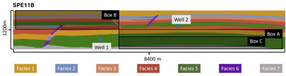
Fig. 16 Schematic representation of SPE11B case and its reporting boxes. Image extracted from arxiv version
Here blue, red and orange boxes are representing the prescribed reporting boxes, respectively denoted box A, B and C from the description. These locations are used to observe the initial accumulation in the first anticline, the accumulation at the top of anticlines due to fluid migration through heterogeneous structures, and the development of convective mixing finger patterns.
Input base
This benchmark test is based on the XML file located below:
inputFiles/compositionalMultiphaseFlow/benchmarks/SPE11/b/spe11b_vti_source_00840x00120.xml
which includes
inputFiles/compositionalMultiphaseFlow/benchmarks/SPE11/b/spe11b_vti_source_base.xml
for all parameters not related to the mesh discretization. The full simulation involves 1000 years of initial thermal equilibration required to let the system stabilize under the geothermal gradient before starting the injection schedule.
The well schedule consists of 50 years of injection for the bottom injector and 25 years with a 25 year delayed start for the top injector. It is then followed by a 950 years of migration, dissolution and convection.
As we can see in the snippet below, SourceFlux was choosen to model the injection (rather than wellbores). It goes with a
FieldSpecification setting for the temperature at the same place to define the imposed injected CO2 temperature. This also includes to object
defined elsewhere as a set thermalSources1 (respectively thermalSources2) and a Function that varies over time to represent the flux schedule.
These will be discussed in more details below.
    <FieldSpecification
      beginTime="0.01"
      endTime="1.5768e9"
      name="sourceTemperature1"
      setNames="{ thermalSource1 }"
      objectPath="ElementRegions"
      fieldName="temperature"
      scale="283.15" />
    <SourceFlux
      name="sourceTerm1"
      objectPath="ElementRegions"
      component="0"
      functionName="totalRateTable1"
      scale="1"
      setNames="{ thermalSource1 }" />

    <FieldSpecification
      beginTime="7.8840000001e8"
      endTime="1.5768e9"
      name="sourceTemperature2"
      setNames="{ thermalSource2 }"
      objectPath="ElementRegions"
      fieldName="temperature"
      scale="283.15" />
    <SourceFlux
      name="sourceTerm2"
      objectPath="ElementRegions"
      component="0"
      functionName="totalRateTable2"
      scale="1"
      setNames="{ thermalSource2 }" />
  </FieldSpecifications>
Constitutives and includes
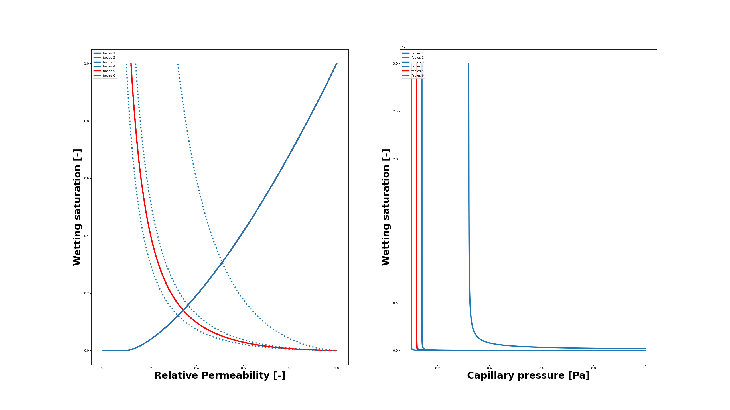
The capillary and residual trapping in such a multi-facies reservoir occur due to the heterogeneous properties. For instance, a large entry pressure jump exists between anticline facies #5 and the upper layers. The box A is chosen such that it can monitor the expected trapped CO2 dissolution. The dissolved CO2 makes the brine heavier which results in its sinking and starts the convective mixing instabilites.
Below we show the sets of relative permeabilities (left) and capillary pressure (right) produced from their tabulated values. The facies #5 is highlighted as it plays an important role in the overall trapping.
The tables import in the simulation deck is done as the following showing the relative permeability and capillary pressure tables for facies #5:
    <TableFunction
      name="waterRelativePermeabilityTable5"
      coordinateFiles="{ ../tables/waterSaturation_spe11b_5.txt }"
      voxelFile="../tables/waterRelperm_spe11b_5.txt"/>
    <TableFunction
      name="gasRelativePermeabilityTable5"
      coordinateFiles="{ ../tables/gasSaturation_spe11b_5.txt }"
      voxelFile="../tables/gasRelperm_spe11b_5.txt"/>
    <TableFunction
      name="cappresTable5"
      coordinateFiles="{ ../tables/waterPCSaturation_spe11b_5.txt}"
      voxelFile="../tables/waterCapPres_spe11b_5.txt"/>
Then, relative permeabilities and capillary pressure are defined under the Constitutive tag. For example, the relative permeability for the facies #1 is defined as
    <TableRelativePermeability
      name="relperm1"
      phaseNames="{ gas, water }"
      wettingNonWettingRelPermTableNames="{ waterRelativePermeabilityTable1, gasRelativePermeabilityTable1 }" />
Other properties such as permeabilities, diffusivity, and rock thermal conductivity are modeled as constant per facies (thermal conductivity definition is shown as an example):
    <MultiPhaseVolumeWeightedThermalConductivity
      name="thermalCond"
      phaseNames="{ gas, water }"
      phaseThermalConductivity="{ 0.09, 0.65 }"
      rockThermalConductivityComponents="{ 1.25, 1.25, 1.25 }" />
In addition, the scaling of the Constitutive values is defined to represent the facies:
    <FieldSpecification
      name="condx1"
      initialCondition="1"
      component="0"
      setNames="{ all }"
      objectPath="ElementRegions/reservoir1"
      fieldName="thermalCond_rockThermalConductivity"
      scale="1.9" />
    <FieldSpecification
      name="condy1"
      initialCondition="1"
      component="1"
      setNames="{ all }"
      objectPath="ElementRegions/reservoir1"
      fieldName="thermalCond_rockThermalConductivity"
      scale="1.9" />
Note
Their FieldSpecification scaling definition is linked to the Constitutive definition through the generated field name, for instance thermalCond_rockThermalConductivity. The prefix being extracted from the Constitutive name attributes.
The permeabilities and porosities are defined similarly to the rock thermal conductivities using the scaling approach. The diffusivity being non-heterogeneous in the specifications of the case, it is solely defined in its Constitutive model.
Eventually, one has to pick a model for both brine and CO2 densities and viscosities with respect to varying pressure, temperature and composition. It is done using the CO2BrinePhillipsThermalFluid tag. It lists files that include the related parameters. For instance, CO2 density is modeled through Span Wagner model, while the viscosities are obtained via Fenghour model (see CO2-brine model for more details).
    <CO2BrinePhillipsThermalFluid
      name="fluid"
      phaseNames="{ gas, water }"
      logLevel="0"
      componentNames="{ co2, water }"
      componentMolarWeight="{ 44e-3, 18e-3 }"
      phasePVTParaFiles="{ tables/pvtgas_thermal.txt, tables/pvtliquid_thermal.txt }"
      flashModelParaFile="tables/co2flash_thermal.txt" />
The model conformity to NIST values is assessed in the following plots:
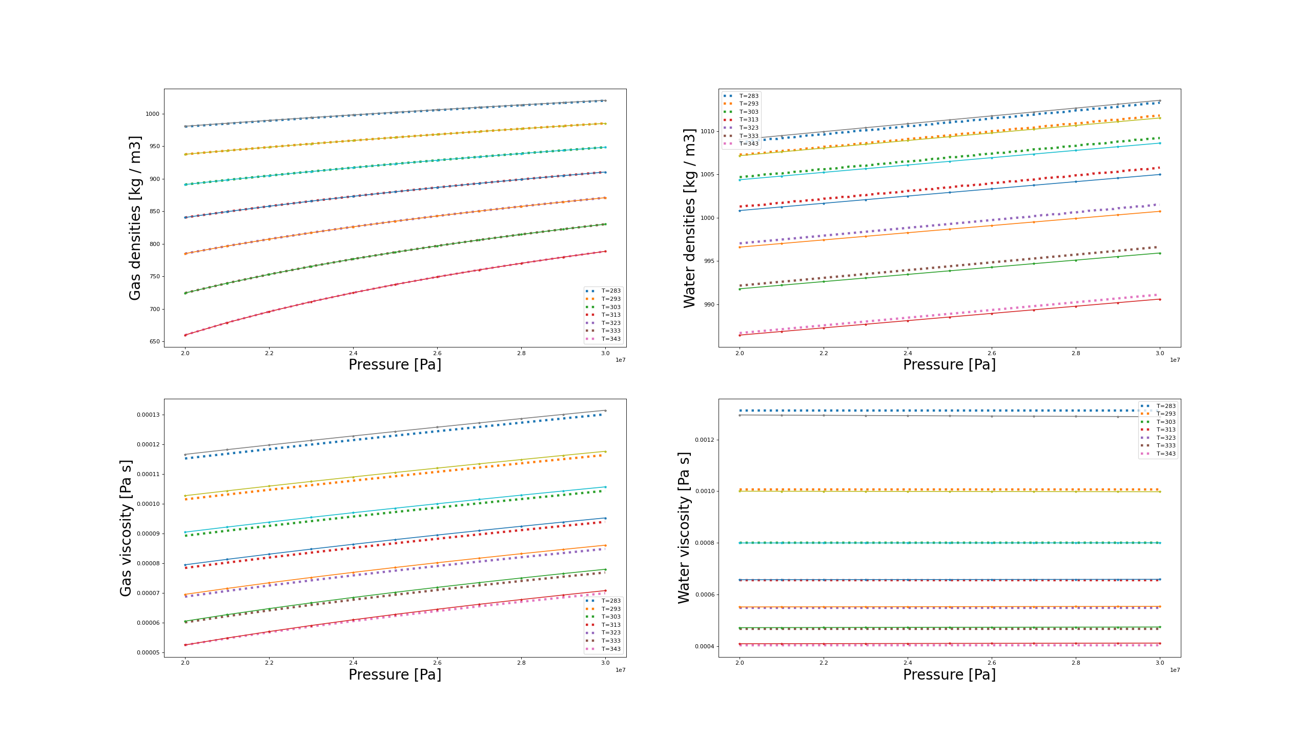
Fluid model comparison with NIST data. The dotted lines represent GEOS values while the solid-and-stars are the values from NIST database.
The plots demonstrate the validity of the selected models with respect to the provided NIST tables over the range of pressures and temperatures.
Flow solver
The CompositionalMultiphaseFVM solver uses the finite volume discretization on the targetRegions. The discretization will be TPFA
  <NumericalMethods>
    <FiniteVolume>
      <TwoPointFluxApproximation
        name="fluidTPFA" />
    </FiniteVolume>
  </NumericalMethods>
and here is linked-by-name to the TwoPointFluxApproximation XML block. The Phase Potential Upwind (PPU) scheme is used.
  <Solvers>
    <CompositionalMultiphaseFVM
      name="compositionalMultiphaseFlow"
      targetRegions="{ reservoir1, reservoir2, reservoir3, reservoir4, reservoir5, reservoir6, reservoir7 }"
      discretization="fluidTPFA"
      temperature="333.15"
      isThermal="1"
      initialDt="1e2"
      targetPhaseVolFractionChangeInTimeStep="0.2"
      maxCompFractionChange="0.2"
      logLevel="1"
      useMass="1">
      <NonlinearSolverParameters
        newtonTol="1.0e-4"
        maxTimeStepCuts="100"
        maxSubSteps="1000"
        lineSearchAction="Attempt"
        lineSearchStartingIteration="5"
        timeStepIncreaseIterLimit="0.3"
        timeStepDecreaseIterLimit="0.6"
        newtonMaxIter="15" />
      <LinearSolverParameters
        solverType="fgmres"
        preconditionerType="mgr"
        krylovTol="1e-5"
        krylovMaxIter="100"
        logLevel="1" />
    </CompositionalMultiphaseFVM>
  </Solvers>
Note the important isThermal and useMass flags are enabled. The targetPhaseVolFractionChangeInTimeStep parameter controls the time step selection and the maxCompFractionChange parameter controls the solution chopping strategy in the solver. The NonlinearSolverParameters contains the nonlinear tolerance, line search parameters, and the parameters for the time step increase and decrease. The LinearSolverParameters contains parameters for the linear solver: the standard pick here is Flexible GMRES iterative solve with Multi Grid Reduction preconditioner.
Initial and boundary conditions
In the following, we will provide more details about the initialization and describe how to set both the injections and the left and right buffers used to mimic large connected aquifers.
As mentioned above, the injection description refers to a cell set to be applied on and a Function defining incoming flux over time.
The cell sets are defined using boxes in the discretization-specific file (also root file):
  <Geometry>
    <Box
      name="top"
      xMin="{   -0.01, -0.01, 1189.99 }"
      xMax="{ 8400.01,  1.01, 1200.01 }" />
    <Box
      name="bottom"
      xMin="{   -0.01, -0.01, -0.01 }"
      xMax="{ 8400.01,  1.01, 10.01 }" />
      <Box
       name="thermalSource1"
       xMin="{ 2699.99, -0.01, 299.99 }"
       xMax="{ 2710.01,  1.01, 310.01 }" />
      <Box
       name="thermalSource2"
       xMin="{ 5099.99, -0.01, 699.99 }"
       xMax="{ 5110.01,  1.01, 710.01 }" />
  </Geometry>
The lower-interpolated 1D function over time serve as a scaler for the incoming flux:
  <Functions>
    <TableFunction
      name="initCO2CompFracTable"
      coordinates="{ 0, 1200 }"
      values="{ 0.0, 0.0 }" />
    <TableFunction
      name="initWaterCompFracTable"
      coordinates="{ 0, 1200 }"
      values="{ 1.0, 1.0 }" />
    <TableFunction
      name="initTempTable"
      coordinates="{ 0, 1200 }"
      values="{ 343.15, 313.15 }" />

    <TableFunction
      name="totalRateTable1"
      inputVarNames="{ time }"
      coordinates="{ -1e11, 0, 7.884e8, 1.5768e9, 1.576800001e9, 3.153600e10 }"
      values="{ 0, -0.035, -0.035, -0.035, 0, 0}"
      interpolation="lower" />
    <TableFunction
      name="totalRateTable2"
      inputVarNames="{ time }"
      coordinates="{ -1e11, 0, 7.8839999e8, 7.884e8, 1.5768e9, 1.576800001e9, 3.153600e10 }"
      values="{ 0., 0., 0., -0.035, -0.035, 0, 0}"
      interpolation="lower" />
  </Functions>
Note
Note that the units here are in mass as the useMass=1 attribute is set in Solvers.
Using Functions we also imposed the initial geothermal gradient as well as initial compositions. Then we need to define the HydrostaticEquilibrium to be computed, as shown below:
  <FieldSpecifications>
    <HydrostaticEquilibrium
      name="equil"
      objectPath="ElementRegions"
      datumElevation="300"
      datumPressure="3e7"
      initialPhaseName="water"
      componentNames="{ co2, water }"
      componentFractionVsElevationTableNames="{ initCO2CompFracTable, initWaterCompFracTable }"
      temperatureVsElevationTableName="initTempTable" />
Finally, the the equilibration stage is defined in the Events by setting the simulation to start at -1000 years:
  <Events
    minTime="-31536000000"
    maxTime="31536000000">

    <PeriodicEvent
      name="solverApplications0"
      beginTime="-31536000000"
      maxEventDt="157680000"
      endTime="0"
      target="/Solvers/compositionalMultiphaseFlow" />
    <PeriodicEvent
      name="solverApplications1"
      beginTime="0"
      maxEventDt="2.6e5"
      endTime="7.884e5"
      target="/Solvers/compositionalMultiphaseFlow" />
    <PeriodicEvent
      name="solverApplications2"
      beginTime="7.884e5"
      maxEventDt="1.3e6"
      target="/Solvers/compositionalMultiphaseFlow" />
Note
The time tags in GEOS are in seconds. Here a split between equilibration, start of the injection and post-injection is chosen as
the maximum time steps in these stages are quite different. Specifically, separate solverApplication1 definition is ensuring stability as the injection starts.
The boundary conditions for the domain are imposed as follows. The top and bottom temperatures are set using the FieldSpecification on top and bottom geometrical sets defined above:
<Problem>
  <FieldSpecifications>
    <FieldSpecification
      name="topTemperature"
      objectPath="ElementRegions"
      fieldName="temperature"
      scale="313.15"
      setNames="{ top }" />
    <FieldSpecification
      name="bottomTemperature"
      objectPath="ElementRegions"
      fieldName="temperature"
      scale="343.15"
      setNames="{ bottom }" />
</FieldSpecifications>

</Problem>
Fictive aquifers are used as buffers to damp the pressure buildup
(see (Nordbotten et al.,2024), for details about these buffers definition).
They are set similar to the sources definition but instead of using the boxes for cell sets,
we use tags created during the construction of the mesh, namely 12_hexahedra to 15_hexahedra. It is then easy to
rescale the volumes in those regions:
    <FieldSpecification
      name="vol12"
      initialCondition="1"
      setNames="{ all }"
      objectPath="ElementRegions/reservoir2/12_hexahedra"
      fieldName="elementVolume"
      functionName="bufferVolume"
      scale="1.0" />
    <FieldSpecification
      name="vol13"
      initialCondition="1"
      setNames="{ all }"
      objectPath="ElementRegions/reservoir3/13_hexahedra"
      fieldName="elementVolume"
      functionName="bufferVolume"
      scale="1.0" />
    <FieldSpecification
      name="vol14"
      initialCondition="1"
      setNames="{ all }"
      objectPath="ElementRegions/reservoir4/14_hexahedra"
      fieldName="elementVolume"
      functionName="bufferVolume"
      scale="1.0" />
    <FieldSpecification
      name="vol15"
      initialCondition="1"
      setNames="{ all }"
      objectPath="ElementRegions/reservoir5/15_hexahedra"
      fieldName="elementVolume"
      functionName="bufferVolume"
      scale="1.0" />
The scaling factor depends on the discretization and hence that is defined in the discretization-specific file:
  <Functions>
    <TableFunction
      name="bufferVolume"
      inputVarNames="{ time }"
      coordinates="{ -1e11 }"
      values="{ 500100 }"
      interpolation="lower" />
  </Functions>
Post-processing and reporting
First, inspection of the results is done using Paraview as in the usual GEOS workflow. Here, we report temperature, saturation and dissolved CO2 fraction for 500 years and 1000 years:
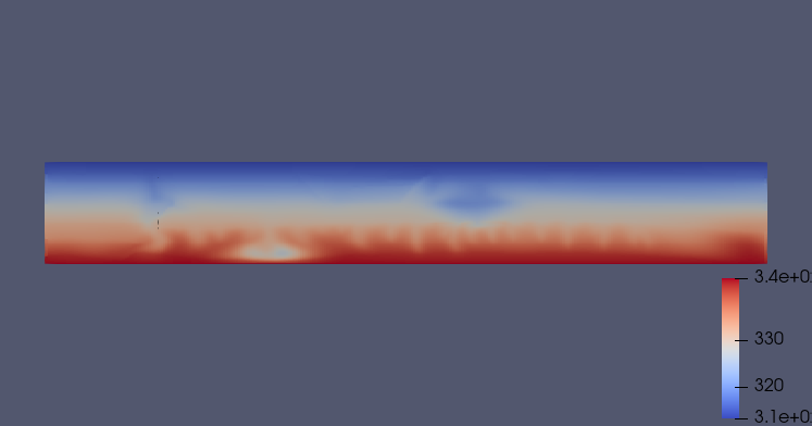
Fig. 17 Thermal state after 500 years
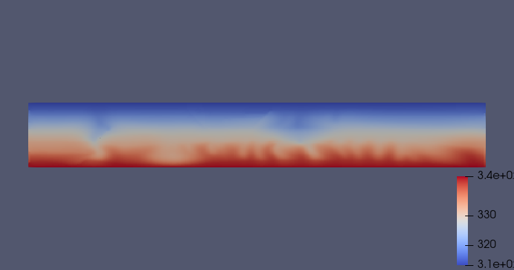
Fig. 18 Thermal state after 1000 years
The saturation distribution is showing that, for this mesh resolution, almost all gaseous CO2 is trapped and then dissolved after 1000 years of the injection scenario. The reporting of the dissolved fraction clearly shows evidence of on-set of convective mixing fingers, with heavier CO2-saturated brine sinking. In particular, the dissolved CO2 sinks and accumulates in the lower left part of the domain, perpendicular to the first injector. This behavior is similar for the temperature distributions.
GEOS run can be post-treated leveraging Paraview (as mentioned in other tutorials) or pyvtk. Here is an example of the latter. It is built around two main driver write() and plot() functions which respectively write the integrated mass balance in the reporting boxes A and B and re-read the generated file and plot it to png. It requires usual dependencies such as re, os, pandas, numpy, scipy (for interpolation) and pyplot
import os, logging
import numpy as np
import pandas as pd
import matplotlib.pyplot as plt
in addition to pyvtk. The main drivers hereafter,
def write(ifile):

    #utils
    def read_pvd(ifile):

        logging.info(f'Reading pvd file {ifile}')
        import xml.etree.ElementTree as ET
        tree = ET.parse(ifile)
        root = tree.getroot()
        for ds in root.find('Collection').findall('DataSet'):
            data.data_sets[float(ds.attrib['timestep'])] = ds.attrib['file']


    # note that solubility is in KgCO2/KgBrine
    read_pvd(ifile)
    define_boxes()
    # preprocess input list from desired output
    import re
    olist_ = set(
        [item for name in name_indirection.keys() for item in re.findall(r'(\w+)_\d|(\w+)', name)[0] if
         len(item) > 0])

    ddf = pd.DataFrame()
    for time in data.schedule:
        field_and_pts = process_time(ifile, time, olist_)
        ddf = pd.concat([ddf, intergrate_fields(field_and_pts)])
    ddf.to_csv( './spe11b_time_series.csv',
                       index_label=False)


def plot():
    df = pd.read_csv('./spe11b_time_series.csv')
    fig, axs = plt.subplots(2, 2)
    (time_name, time_unit), (mass_name, mass_unit), (pressure_name, pressure_unit) \
        = ('Y', SEC2YEAR), ('T', 1000), ('bar', 1e5)
    # pressures
    axs[0][0].plot(df['t[s]'].to_numpy() / time_unit, df['p1[Pa]'].to_numpy() / pressure_unit,
                   label=f'pressure 1 [{pressure_name}]')
    axs[0][0].plot(df['t[s]'].to_numpy() / time_unit, df['p2[Pa]'].to_numpy() / pressure_unit,
                   label=f'pressure 2 [{pressure_name}]')
    axs[0][0].legend()
    # box A
    axs[0][1].plot(df['t[s]'].to_numpy() / time_unit, df['mobA[kg]'].to_numpy() / mass_unit,
                   label=f'mobile CO2 [{mass_name}]')
    axs[0][1].plot(df['t[s]'].to_numpy() / time_unit, df['immA[kg]'].to_numpy() / mass_unit,
                   label=f'immobile CO2 [{mass_name}]')
    axs[0][1].plot(df['t[s]'].to_numpy() / time_unit, df['dissA[kg]'].to_numpy() / mass_unit,
                   label=f'dissolved CO2 [{mass_name}]')
    axs[0][1].legend()
    axs[0][1].set_title('boxA')
    # box B
    axs[1][0].plot(df['t[s]'].to_numpy() / time_unit, df['mobB[kg]'].to_numpy() / mass_unit,
                   label=f'mobile CO2 [{mass_name}]')
    axs[1][0].plot(df['t[s]'].to_numpy() / time_unit, df['immB[kg]'].to_numpy() / mass_unit,
                   label=f'immobile CO2 [{mass_name}]')
    axs[1][0].plot(df['t[s]'].to_numpy() / time_unit, df['dissB[kg]'].to_numpy() / mass_unit,
                   label=f'dissolved CO2 [{mass_name}]')
    axs[1][0].legend()
    axs[1][0].set_title('boxB')

    fig.tight_layout()
    fig.savefig('./spe11b_timeseries.png', bbox_inches='tight')


if __name__ == "__main__":

    write('vtkOutput.pvd')
    # plot
    plot()
are using simple data structure to gather info and to link GEOS’ name to name used in formulas,
# for geos
name_indirection = {'pressure': 'pres',
                         'phaseVolumeFraction_0': 'satg',
                         'phaseVolumeFraction_1': 'satw',
                         'fluid_phaseCompFraction_2': 'mCO2',
                         'fluid_phaseCompFraction_1': 'mH2O',
                         'fluid_phaseDensity_0': 'rG',
                         'fluid_phaseDensity_1': 'rL',
                         'rockPorosity_porosity': 'poro',
                         'elementVolume': 'vol',
                         'phaseMobility_0': 'krg',
                         'phaseMobility_1': 'krw'}

logging.basicConfig(filename='spe11-pt.log', encoding='utf-8', level=logging.INFO)


SEC2YEAR =  365*24*3600

#main containers
class Data:

    data_sets = {}
    schedule = []
    PO1 = []
    PO2 = []
    boxes = {}

data = Data()
def define_boxes():
    #define and rescale
    data.boxes = {'Whole': [(0.0, 0.0, 0.0), (8400, 1., 1200.)]}

    data.boxes['A'] = [(3300.,0.,0.), (8300.,1.,600.)]
    data.boxes['B'] = [(100.,0.,600.), (3300.,1.,1200.)]
    data.PO1 = [ 4500, 500]
    data.PO2 = [ 5100, 1100]
    data.schedule = np.arange(0., 1000 * SEC2YEAR, 1000/200 * SEC2YEAR)
It uses a string interpreted function process_keys(formula, fielddict) to build the observable from the fields loaded from GEOS :
formula = {'mImmobile': 'if(krg<0.001, rG*satg*poro*vol)',
           'mMobile': 'if(krg>0.001,rG*satg*poro*vol)',
           'mDissolved': 'rL*mCO2*poro*vol*satw' }
def process_keys(formula, fielddict):
    """
    Basic formula interface, reading from multiplication and division (no parenthesis)
    :param formula: string of the formula
    :param fielddict: all-containing dict with base-variables
    :return: Array of the formula value
    """
    import re
    if re.findall(r'if', formula):
        bits = formula.split(',')
        assert (len(bits) == 2)
        cdt = bits[0][3:]
        if re.findall(r'>', cdt):
            inner_bits = cdt.split('>')
            cdt_field = inner_bits[0].strip()
            cdt_lim = float(inner_bits[1])
            return np.where(fielddict[cdt_field] > cdt_lim, process_keys(bits[1][:-1], fielddict), 0)
        elif re.findall(r'<', cdt):
            inner_bits = cdt.split('<')
            cdt_field = inner_bits[0].strip()
            cdt_lim = float(inner_bits[1])
            return np.where(fielddict[cdt_field] < cdt_lim, process_keys(bits[1][:-1], fielddict), 0)
        else:
            raise NotImplemented('Not a valid condition')
    elif re.findall(r'\+', formula):
        bits = formula.split('+')
        bits = [item.strip() for item in bits]
        return process_keys(bits[0], fielddict) + process_keys('+'.join(bits[1:]), fielddict)
    elif re.findall(r'-', formula):
        bits = formula.split('-')
        bits = [item.strip() for item in bits]
        return process_keys(bits[0], fielddict) - process_keys('+'.join(bits[1:]), fielddict)
    elif re.findall(r'\*', formula):
        bits = formula.split('*')
        bits = [item.strip() for item in bits]
        return process_keys(bits[0], fielddict) * process_keys('*'.join(bits[1:]), fielddict)
    elif re.findall(r'/', formula):
        bits = formula.split('/')
        bits = [item.strip() for item in bits]
        return process_keys(bits[0], fielddict) / process_keys('/'.join(bits[1:]), fielddict)
    return fielddict[formula]
and a tool set to interpolate and integrate them over the correct boxes,
def get_interpolate(points_from_vtk, fields: dict, nskip=1):
    """ getting dict of proper interpolation for fields """
    def get_lambda_2(xpts, disc_func):
        from scipy.interpolate import LinearNDInterpolator
        x, z = xpts
        return LinearNDInterpolator(np.asarray([x, z]).transpose(), disc_func, fill_value=0.0)

    fn = {}
    for key, val in fields.items():
        if key in name_indirection.values() or key in formula.keys():
            logging.info(f'Building interpolation for {key}')
            # do not interpolate if not interested by (and only brought as field is another component of
            # a field of interest
            T = points_from_vtk
            fn[key] = get_lambda_2((T[::nskip, 0], T[::nskip, 2]), val[::nskip])

    return fn

def integrate_2(pts, fields, box):
    """ Simplistic integration equivalent to Paraview integrate variables """
    xmin, ymin, zmin = box[0]
    xmax, ymax, zmax = box[1]
    ii = np.intersect1d(np.intersect1d(np.argwhere((pts[:, 0] > xmin)), np.argwhere((pts[:, 0] < xmax))),
                        np.intersect1d(np.argwhere((pts[:, 2] > zmin)), np.argwhere((pts[:, 2] < zmax))))
    return fields[ii].sum()

def intergrate_fields(pft_tuple: list):

    logging.info(f'Interpolating reported fields')
    lines = list()
    pts_from_vtk, fields, time = pft_tuple

    # some lines for MC magic number
    for key, form in formula.items():
        fields[key] = process_keys(form, fields)

    fn = get_interpolate(pts_from_vtk,
                                    {'pres': fields['pres'], 'vol': fields['vol']},
                                    nskip=1)

    line = [time]
    logging.info(f'Writing sparse time {time:2}')
    # deal with P1 and P2
    p1 = fn['pres'](data.PO1)
    p2 = fn['pres'](data.PO2)
    line.extend([p1[0], p2[0]])
    # deal box A & B
    logging.info(f'Integrating for boxes A and B')
    for box_name, box in data.boxes.items():
            if box_name in ['A', 'B']:
                line.extend([
                    integrate_2(pts_from_vtk, fields['mMobile'], box),
                    integrate_2(pts_from_vtk, fields['mImmobile'], box),
                    integrate_2(pts_from_vtk, fields['mDissolved'], box)
                ])
        # #deal sealTot
    lines.append(line)

    return pd.DataFrame(data=lines,
                        columns=['t[s]', 'p1[Pa]', 'p2[Pa]', 'mobA[kg]', 'immA[kg]', 'dissA[kg]',
                                 'mobB[kg]', 'immB[kg]', 'dissB[kg]'])
Eventually, the per-time driver, load usefull specific fields from the correct time in the multi-block VTK format GEOS is using,
def process_time(pvdfile, time, olist):

    import vtk
    import numpy as np
    from vtk.util import numpy_support

    reader = vtk.vtkXMLMultiBlockDataReader()
    reader.SetFileName( './' + os.path.dirname(pvdfile) + '/' + data.data_sets[time] )
    loadlist = list(olist)

    for fieldname in loadlist:
        if fieldname in olist or fieldname in ['ghostRank']:
            reader.SetCellArrayStatus(fieldname, 1)
        else:
            reader.SetCellArrayStatus(fieldname, 0)

    logging.info('Updating multiblocks')
    reader.Update()
    logging.info('Processing multiblocks')
    # remove well blocks - in hierarchy mesh.lvl0.CellElementRegion/WellElementRegion
    if reader.GetOutput().GetBlock(0).GetBlock(0).GetNumberOfBlocks() > 1:
        reader.GetOutput().GetBlock(0).GetBlock(0).RemoveBlock(1)

    # browse blocks - assemble size
    # counting cells and blocks/rank
    nv = reader.GetOutput().GetNumberOfCells()
    it = reader.GetOutput().NewIterator()
    it.InitTraversal()

    ncnf = 0
    it = reader.GetOutput().NewIterator()
    it.InitTraversal()
    for ifields in olist:
        ncc = reader.GetOutput().GetDataSet(it).GetCellData().GetArray(ifields).GetNumberOfComponents()
        ncnf += ncc
        it.GoToNextItem()

    # form data container
    f = np.zeros(shape=(nv, ncnf), dtype='float')
    pts = np.zeros(shape=(nv, 3), dtype='float')

    # get seal flagged
    mesh = reader.GetOutput().GetBlock(0).GetBlock(0).GetBlock(0)
    fielddict = {}
    for i in range(0, mesh.GetNumberOfBlocks()):
        start = 0
        it = mesh.GetBlock(i).NewIterator()
        it.InitTraversal()
        info = mesh.GetMetaData(i)
        while not it.IsDoneWithTraversal():
            field = mesh.GetBlock(i).GetDataSet(it).GetCellData().GetArray("ghostRank")
            it.GoToNextItem()

        nc = 0
        j = 0  # for field loop
        for ifields in olist:
            start = 0
            it = reader.GetOutput().NewIterator()
            it.InitTraversal()
            while not it.IsDoneWithTraversal():
                field = reader.GetOutput().GetDataSet(it).GetCellData().GetArray(ifields)
                nt = field.GetNumberOfValues()
                nc = field.GetNumberOfComponents()
                f[start:(start + int(nt / nc)), j:j + nc] = numpy_support.vtk_to_numpy(field).reshape(int(nt / nc),
                                                                                                      nc)

                cc = vtk.vtkCellCenters()
                cc.SetInputData(reader.GetOutput().GetDataSet(it))
                cc.Update()
                if nt > 0:
                    pts[start:(start + int(nt / nc)), :] = numpy_support.vtk_to_numpy(
                        cc.GetOutput().GetPoints().GetData())
                it.GoToNextItem()
                start += int(nt / nc)

            if nc > 1:
                for k in range(0, nc):
                    if ifields + "_" + str(k) in name_indirection:
                        fielddict[name_indirection[ifields + "_" + str(k)]] = f[:, j + k]
            else:
                if ifields in name_indirection:
                    fielddict[name_indirection[ifields]] = f[:, j]
            j = j + nc

    return pts, fielddict, time
and this function is mapped over the schedule of the simulation.
To go further
Feedback on this example
For any feedback on this example, please submit a GitHub issue on the project’s GitHub page.