Model Initialization: User Defined Tables

Context

This example uses the same reservoir model as the gravity-induced hydrostatic stress initialization case (see Model Initialization: Hydrostatic and Mechanical Equilibrium). Instead of using the gravity based equilibrium initialization procedure, we collect the interpretated stress and pore pressure gradients for a reservoir and then request the simulator to perform an initialization with the provided pressure and stresses in every element in the model. The problem is solved by using the single-phase poromechanics solver (see Poromechanics Solver) in GEOS.

Input file

The xml input files for the test case are located at:

inputFiles/initialization/userdefinedStress_initialization_base.xml
inputFiles/initialization/userdefinedStress_initialization_benchmark.xml

This example also uses a set of table files located at:

inputFiles/initialization/userTables/

Last, a Python script for post-processing the results is provided:

src/coreComponents/physicsSolvers/multiphysics/docs/userTableStressInitialization/tableInitializationFigure.py

Stress Initialization Table Functions

The major distinction between this “user-defined” initialization and the “gravity-based” initialization is that in the user-defined case, the user provides the following additional information:

• The distribution of effective stresses and pore pressure across the domain, with their gradients assumed constant along the depth in this example. We use a table function (see Functions) to specify pressure and stress conditions throughout the area.

This is shown in the following tags under the FieldSpecifications section below

    <FieldSpecification 
      component="0" 
      fieldName="rockSolid_stress" 
      functionName="sigma_xx"
      initialCondition="1" 
      name="init_sigma_xx" 
      objectPath="ElementRegions/Domain" 
      scale="1.0"
      setNames="{ all }" />

    <FieldSpecification
      component="1" 
      fieldName="rockSolid_stress" 
      functionName="sigma_yy"
      initialCondition="1" 
      name="init_sigma_yy" 
      objectPath="ElementRegions/Domain" 
      scale="1.0"
      setNames="{ all }" />

    <FieldSpecification 
      component="2" 
      fieldName="rockSolid_stress" 
      functionName="sigma_zz"
      initialCondition="1" 
      name="init_sigma_zz" 
      objectPath="ElementRegions/Domain" 
      scale="1.0"
      setNames="{ all }" />

    <FieldSpecification 
      fieldName="pressure" 
      functionName="init_pressure" 
      initialCondition="1"
      name="init_pressure" 
      objectPath="ElementRegions/Domain" 
      scale="1.0" 
      setNames="{ all }" />

The tables for sigma_xx, sigma_yy, sigma_zz and init_pressure are listed under the Functions section as shown below.

  <Functions>

    <TableFunction 
      coordinateFiles="{userTables/x.csv, userTables/y.csv, userTables/z.csv}"
      inputVarNames="{elementCenter}" 
      interpolation="linear" 
      name="sigma_xx"
      voxelFile="userTables/effectiveSigma_xx.csv" />

    <TableFunction 
      coordinateFiles="{userTables/x.csv, userTables/y.csv,userTables/z.csv}"
      inputVarNames="{elementCenter}" 
      interpolation="linear" 
      name="sigma_yy"
      voxelFile="userTables/effectiveSigma_yy.csv" />

    <TableFunction 
      coordinateFiles="{userTables/x.csv, userTables/y.csv, userTables/z.csv}"
      inputVarNames="{elementCenter}" 
      interpolation="linear" 
      name="sigma_zz"
      voxelFile="userTables/effectiveSigma_zz.csv" />

    <TableFunction 
      coordinateFiles="{userTables/x.csv, userTables/y.csv, userTables/z.csv}"
      inputVarNames="{elementCenter}" 
      interpolation="linear" 
      name="init_pressure"
      voxelFile="userTables/porePressure.csv" />
  </Functions>

The required input files: x.csv, y.csv, z.csv, effectiveSigma_xx.csv, effectiveSigma_yy.csv, effectiveSigma_zz.csv, and porePressure.csv are generated based on the expected stress-gradients in the model.

A Python script to generate these files is provided:

src/coreComponents/physicsSolvers/multiphysics/docs/userTableStressInitialization/genetrateTable.py

In addition to generating the files listed above, the script prints out the corresponding fluid density and rock density based on the model parameters provided. These values are then input into the defaultDensity parameter of the CompressibleSinglePhaseFluid and ElasticIsotropic tags respectively, as shown below:

    <ElasticIsotropic
      name="rockSolid"
      defaultDensity="3302.752294"
      defaultPoissonRatio="0.25"
      defaultYoungModulus="100.0e6" />

    <CompressibleSinglePhaseFluid
      name="water"
      defaultDensity="1019.36799"
      defaultViscosity="0.001"
      referencePressure="0.000"
      referenceDensity="1000"
      compressibility="4.4e-10"
      referenceViscosity="0.001"
      viscosibility="0.0" />

Inspecting Results

In the example, we request vtk output files for time-series (time history). We use paraview to visualize the outcome at the time 0s. The following figure shows the final gradient of pressure and of the effective vertical stress after initialization is completed.

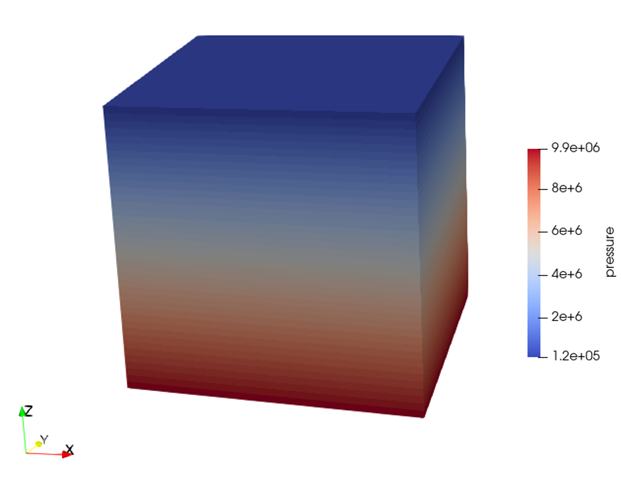
Fig. 93 Simulation result of pressure

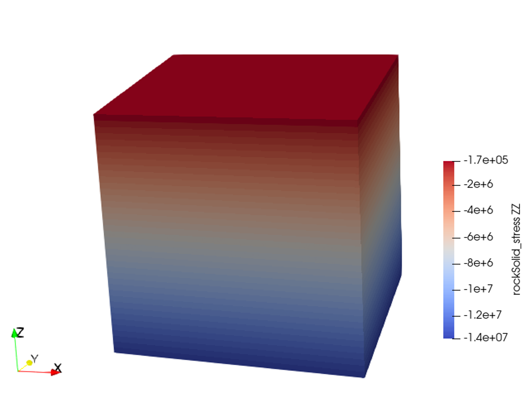
Fig. 94 Simulation result of effective vertical stress

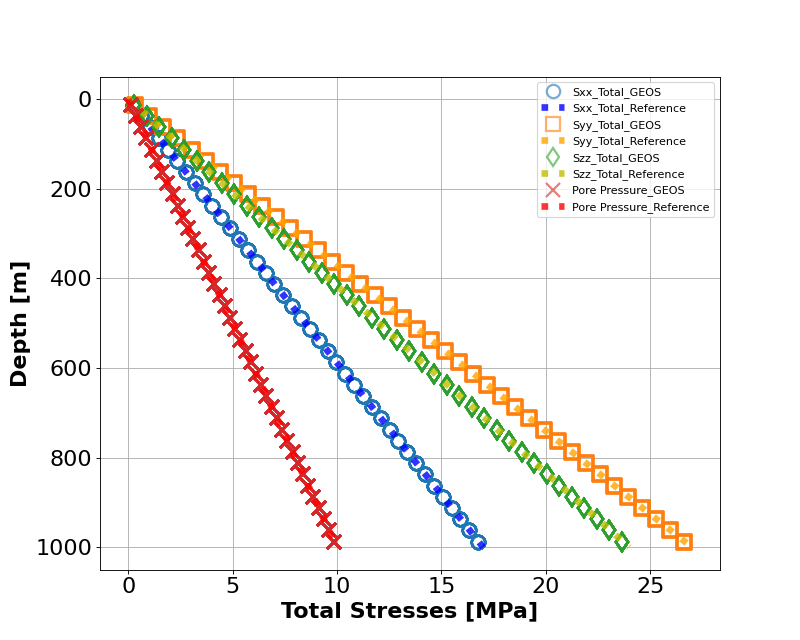
The figure below shows the comparisons between the numerical predictions (marks) and the corresponding user-provided stress gradients. Note that anisotropic horizontal stresses are obtained through this intialization procedure; however, mechanical equilibrium might not be guaranteed, especially for the heterogeneous models.

(Source code)

To go further

Feedback on this example

For any feedback on this example, please submit a GitHub issue on the project’s GitHub page.