Sneddon’s Problem

Objectives

At the end of this example you will know:

how to define fractures in a porous medium,

how to use various solvers (EmbeddedFractures, LagrangianContact and HydroFracture) to solve the mechanics problems with fractures.

Input file

This example uses no external input files and everything required is contained within GEOS input files.

The xml input files for the case with EmbeddedFractures solver are located at:

inputFiles/efemFractureMechanics/Sneddon_embeddedFrac_base.xml
inputFiles/efemFractureMechanics/Sneddon_embeddedFrac_verification.xml

The xml input files for the case with LagrangianContact solver are located at:

inputFiles/lagrangianContactMechanics/Sneddon_base.xml
inputFiles/lagrangianContactMechanics/Sneddon_benchmark.xml
inputFiles/lagrangianContactMechanics/ContactMechanics_Sneddon_benchmark.xml

The xml input files for the case with HydroFracture solver are located at:

inputFiles/hydraulicFracturing/Sneddon_hydroFrac_base.xml
inputFiles/hydraulicFracturing/Sneddon_hydroFrac_benchmark.xml

Description of the case

We compute the displacement field induced by the presence of a pressurized fracture, of length $L_f$ , in a porous medium.

GEOS will calculate the displacement field in the porous matrix and the displacement jump at the fracture surface. We will use the analytical solution for the fracture aperture, $w_n$ (normal component of the jump), to verify the numerical results

$w_n (s) = \frac{4(1 - \nu^2)p_f}{E} \, \sqrt{ \frac{L_f^2}{4} - s^2 }$

where - $E$ is the Young’s modulus - $\nu$ is the Poisson’s ratio - $p_f$ is the fracture pressure - $s$ is the local fracture coordinate in $[-\frac{L_f}{2}, \frac{L_f}{2}]$

In this example, we focus our attention on the Solvers, the ElementRegions, and the Geometry tags.

Mechanics solver

To define a mechanics solver capable of including embedded fractures, we will define a SolidMechanicsEmbeddedFractures solver, called mechSolve. Note that the name attribute of the solver is chosen by the user and is not imposed by GEOS.

Additionally, we need to specify another solver of type, EmbeddedSurfaceGenerator, which is used to discretize the fracture planes.

    <SolidMechanicsEmbeddedFractures
      name="mechSolve"
      targetRegions="{ Domain, Fracture }"
      initialDt="10"
      discretization="FE1"
      logLevel="1"
      contactPenaltyStiffness="0.0e8">
      <NonlinearSolverParameters
        newtonTol="1.0e-6"
        newtonMaxIter="4"
        maxTimeStepCuts="1"/>
      <LinearSolverParameters
        solverType="gmres"
        preconditionerType="mgr"
        logLevel="0"/>
    </SolidMechanicsEmbeddedFractures>

    <EmbeddedSurfaceGenerator
      name="SurfaceGenerator"
      discretization="FE1"
      targetRegions="{ Domain, Fracture }"
      fractureRegion="Fracture"
      targetObjects="{ FracturePlane }"
      logLevel="1"
      mpiCommOrder="1"/>
  </Solvers>

To setup a coupling between rock and fracture deformations in LagrangianContact solver, we define two different solvers:

For solving the frictional contact and rock deformations, we define a Lagrangian contact solver, called here lagrangiancontact. In this solver, we specify targetRegions that include both the continuum region Region and the discontinuum region Fracture where the solver is applied to couple rock and fracture deformations. The contact constitutive law used for the fracture elements is named frictionLaw, and is defined later in the Constitutive section.
The solver SurfaceGenerator defines the fracture region and rock toughness.

    <SolidMechanicsLagrangeContact
      name="lagrangiancontact"
      stabilizationName="TPFAstabilization"
      logLevel="1"
      discretization="FE1"
      targetRegions="{ Region, Fracture }">
      <NonlinearSolverParameters
        newtonTol="1.0e-8"
        logLevel="2"
        newtonMaxIter="10"
        maxNumConfigurationAttempts="10"
        lineSearchAction="Require"
        lineSearchMaxCuts="2"
        maxTimeStepCuts="2"/>
      <LinearSolverParameters
        solverType="direct"
        directParallel="1"
        logLevel="0"/>
    </SolidMechanicsLagrangeContact>
  </Solvers>

Three elementary solvers are combined in the solver Hydrofracture to model the coupling between fluid flow within the fracture, rock deformation, fracture opening/closure and propagation:

Rock and fracture deformation are modeled by the solid mechanics solver SolidMechanicsLagrangianFEM. In this solver, we define targetRegions that includes both the continuum region and the fracture region. The name of the contact constitutive behavior is also specified in this solver by the contactRelationName.
The single phase fluid flow inside the fracture is solved by the finite volume method in the solver SinglePhaseFVM.
The solver SurfaceGenerator defines the fracture region and rock toughness.

    <Hydrofracture
      name="hydrofracture"
      solidSolverName="lagsolve"
      flowSolverName="SinglePhaseFlow"
      surfaceGeneratorName="SurfaceGen"
      logLevel="1"
      targetRegions="{ Fracture }"
      maxNumResolves="2">
      <NonlinearSolverParameters
        newtonTol="1.0e-5"
        newtonMaxIter="20"
        lineSearchMaxCuts="3"/>
      <LinearSolverParameters
        directParallel="0"/>
    </Hydrofracture>

    <SolidMechanicsLagrangianFEM
      name="lagsolve"
      discretization="FE1"
      targetRegions="{ Domain, Fracture }"
      contactRelationName="fractureContact"
      contactPenaltyStiffness="1.0e0"/>

    <SinglePhaseFVM
      name="SinglePhaseFlow"
      discretization="singlePhaseTPFA"
      targetRegions="{ Fracture }"/>

    <SurfaceGenerator
      name="SurfaceGen"
      targetRegions="{ Domain }"
      nodeBasedSIF="1"
      initialRockToughness="10.0e6"
      mpiCommOrder="1"/>

Events

For the case with EmbeddedFractures solver, we add multiple events defining solver applications:

an event specifying the execution of the EmbeddedSurfaceGenerator to generate the fracture elements.
a periodic event specifying the execution of the embedded fractures solver.
three periodic events specifying the output of simulations results.

  <Events
    maxTime="1.0">
    <SoloEvent
      name="preFracture"
      target="/Solvers/SurfaceGenerator"/>

    <PeriodicEvent
      name="solverApplications"
      beginTime="0.0"
      endTime="1.0"
      forceDt="1.0"
      target="/Solvers/mechSolve"/>

    <PeriodicEvent
      name="outputs"
      targetExactTimestep="0"
      target="/Outputs/vtkOutput"/>

    <PeriodicEvent
      name="timeHistoryCollection"
      timeFrequency="1.0"
      targetExactTimestep="0"
      target="/Tasks/displacementJumpCollection" />

    <PeriodicEvent
      name="timeHistoryOutput"
      timeFrequency="1.0"
      targetExactTimestep="0"
      target="/Outputs/timeHistoryOutput"/>    
  </Events>

Similar settings are applied for the other two cases.

Mesh, material properties, and boundary conditions

Last, let us take a closer look at the geometry of this simple problem, if using EmbeddedFractures solver. We use the internal mesh generator to create a large domain ( $40\, m \, \times 40 \, m \, \times 1 \, m$ ), with one single element along the Z axes, 121 elements along the X axis and 921 elements along the Y axis.

  <Mesh>  
    <InternalMesh
      name="mesh1"
      elementTypes="{ C3D8 }"
      xCoords="{ -20, -4, 4, 20 }"
      yCoords="{ -20, -4, 4, 20 }"
      zCoords="{ 0, 1 }"
      nx="{ 10, 101, 10 }"
      ny="{ 10, 901, 10 }"
      nz="{ 1 }"
      cellBlockNames="{ cb1 }"/> 
  </Mesh>

The mesh for the case with LagrangianContact solver was also created using the internal mesh generator, as parametrized in the InternalMesh XML tag. The mesh discretizes the same compational domain ( $40\, m \, \times 40 \, m \, \times 1 \, m$ ) with 300 x 300 x 2 eight-node brick elements in the x, y, and z directions respectively.

  <Mesh>
    <InternalMesh
      name="mesh1"
      elementTypes="{ C3D8 }"
      xCoords="{ -20, -2, 2, 20 }"
      yCoords="{ -20, -2, 2, 20 }"
      zCoords="{ 0, 1 }"
      nx="{ 40, 220, 40 }"
      ny="{ 40, 220, 40 }"
      nz="{ 2 }"
      cellBlockNames="{ cb1 }"/>
  </Mesh>

Similarly, the internal mesh generator was used to discretize the same domain ( $40\, m \, \times 40 \, m \, \times 1 \, m$ ) and generate the mesh for the case with Hydrofracture solver, which contains 280 x 280 x 1 eight-node brick elements in the x, y, and z directions.

  <Mesh>
    <InternalMesh 
      name="mesh1"
      elementTypes="{ C3D8 }"
      xCoords="{ -20, -2, 2, 20 }"
      yCoords="{ -20, -2, 2, 20 }"
      zCoords="{ 0, 1 }"
      nx="{ 40, 200, 40 }"
      ny="{ 40, 200, 40 }"
      nz="{ 1 }"
      cellBlockNames="{ cb1 }"/>    
  </Mesh>

In all the three cases, eight-node hexahedral elements are defined as C3D8 elementTypes, and their collection forms a mesh with one group of cell blocks named here cb1. Refinement is necessary to conform with the fracture geometry specified in the Geometry section.

The parameters used in the simulation are summarized in the following table.

Symbol

Parameter

Units

Value

$K$

Bulk modulus

[GPa]

16.7

$G$

Shear modulus

[GPa]

10.0

$L_f$

Fracture length

[m]

2.0

$p_f$

Fracture pressure

[MPa]

-2.0

Note that the internal fracture pressure has a negative value, due to the negative sign convention for compressive stresses in GEOS.

Material properties and boundary conditions are specified in the Constitutive and FieldSpecifications sections.

Adding a fracture

The static fracture is defined by a nodeset occupying a small region within the computation domain, where the fracture tends to open upon internal pressurization:

The test case with EmbeddedFractures solver:

  <Geometry>
    <Rectangle
      name="FracturePlane"
      normal="{1.0, 0.0, 0.0}"
      origin="{0.0, 0.0, 0.0}"
      lengthVector="{0.0, 1.0, 0.0}"
      widthVector="{0.0, 0.0, 1.0}"
      dimensions="{ 2, 10 }"/>
  </Geometry>

The test case with LagrangianContact solver:

  <Geometry>
    <Rectangle
      name="fracture"
      normal="{1.0, 0.0, 0.0}"
      origin="{0.0, 0.0, 0.0}"
      lengthVector="{0.0, 1.0, 0.0}"
      widthVector="{0.0, 0.0, 1.0}"
      dimensions="{ 2, 10 }"/>

    <Rectangle
      name="core"
      normal="{1.0, 0.0, 0.0}"
      origin="{0.0, 0.0, 0.0}"
      lengthVector="{0.0, 1.0, 0.0}"
      widthVector="{0.0, 0.0, 1.0}"
      dimensions="{ 2, 10 }"/>    
  </Geometry>

The test case with HydroFracture solver:

  <Geometry>
    <Box
      name="fracture"
      xMin="{ -0.01,  -1.01, -0.01 }"
      xMax="{ 0.01,   1.01,  1.01 }"/>

    <Box
      name="source"
      xMin="{ -0.01, -0.11, -0.01 }"
      xMax="{ 0.01,  0.11, 1.01 }"/>

    <Box
      name="core"
      xMin="{ -0.01, -10.01, -0.01 }"
      xMax="{ 0.01,  10.01, 1.01 }"/>
  </Geometry> 

To make these cases identical to the analytical example, fracture propagation is not allowed in this example.

Time history function

In the Tasks section, PackCollection tasks are defined to collect time history information from fields. Either the entire field or specified named sets of indices in the field can be collected. In this example, a task is specified to output fracture aperture (normal opening); however, for different solvers, different fieldName and objectPath should be called:

The test case with EmbeddedFractures solver:

  <Tasks>
    <PackCollection
      name="displacementJumpCollection"
      objectPath="ElementRegions/Fracture/embeddedSurfaceSubRegion"
      fieldName="displacementJump"
      setNames="{all}"/>
  </Tasks>

The test case with LagrangianContact solver:

  <Tasks>
    <PackCollection
      name="displacementJumpCollection"
      objectPath="ElementRegions/Fracture/faceElementSubRegion"
      fieldName="displacementJump"/>     
  </Tasks>

The test case with Hydrofracture solver:

  <Tasks>
    <PackCollection
      name="apertureCollection"
      objectPath="ElementRegions/Fracture/faceElementSubRegion"
      fieldName="elementAperture"/>   
  </Tasks>

These tasks are triggered using the Event manager with a PeriodicEvent defined for these recurring tasks. GEOS writes output files named after the string defined in the filename keyword and formatted as HDF5 files. The TimeHistory file contains the collected time history information from each specified time history collector. This information includes datasets for the simulation time, element center defined in the local coordinate system, and the time history information. A Python script is used to read and plot any specified subset of the time history data for verification and visualization.

Running GEOS

To run these three cases, use the following commands:

path/to/geos -i inputFiles/efemFractureMechanics/Sneddon_embeddedFrac_verification.xml

path/to/geos -i inputFiles/lagrangianContactMechanics/ContactMechanics_Sneddon_benchmark.xml

path/to/geos -i inputFiles/hydraulicFracturing/Sneddon_hydroFrac_benchmark.xml

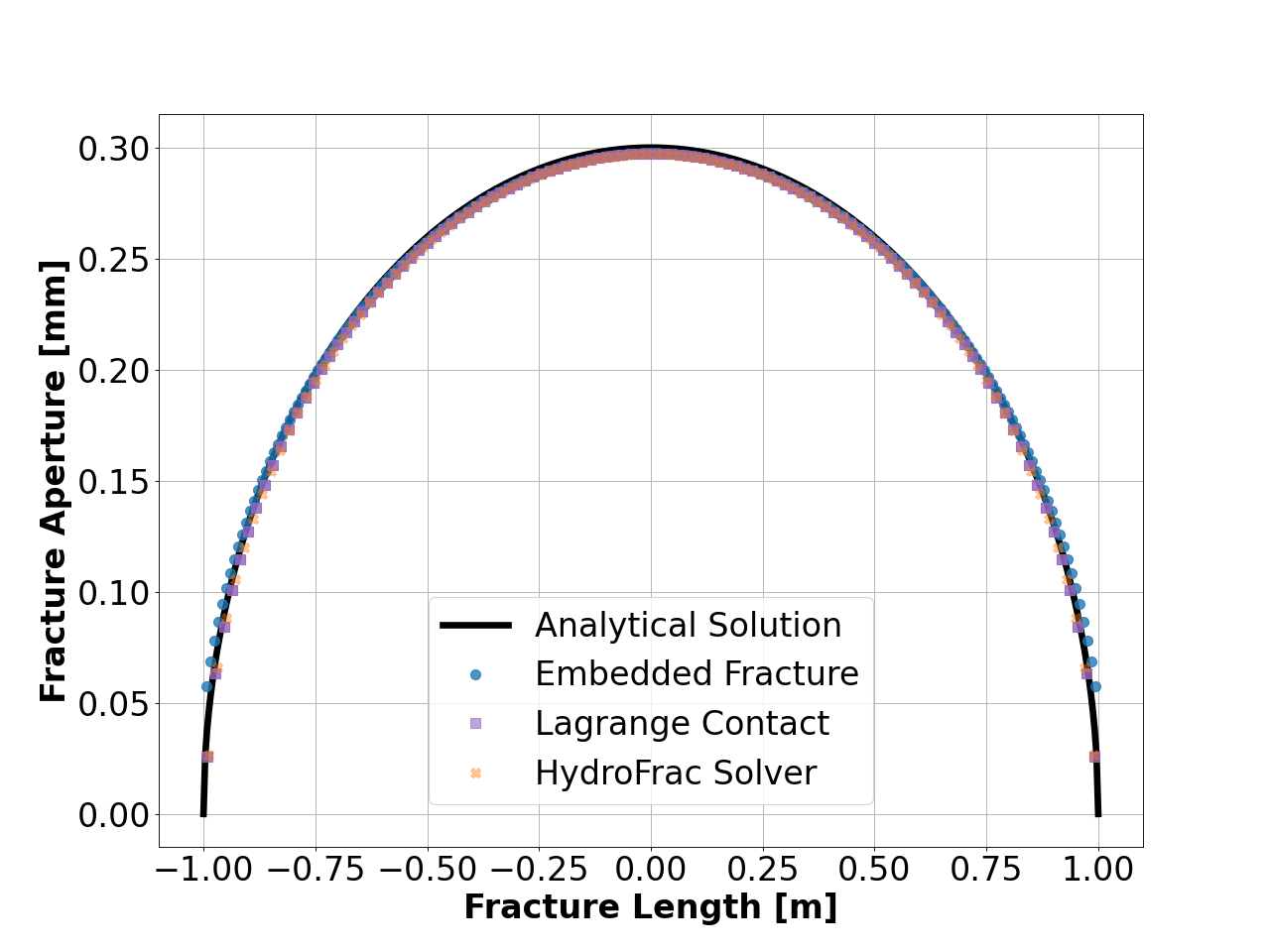
Inspecting results

This plot compares the analytical solution (continuous lines) with the numerical solutions (markers) for the normal opening of the pressurized fracture. As shown below, consistently, numerical solutions with different solvers correlate very well with the analytical solution.

(Source code)

../../../../../../_images/sneddonFigure.png

To go further

Feedback on this example

This concludes the Sneddon example. For any feedback on this example, please submit a GitHub issue on the project’s GitHub page.