Modified Cam-Clay Model for Wellbore Problems
Context
In this benchmark example, the Modified Cam-Clay model (see Model: Modified Cam-Clay) is applied to solve for elastoplastic deformation within the vicinity of a vertical wellbore. For the presented example, an analytical solution is employed to verify the accuracy of the numerical results. The resulting model can be used as a base for more complex analysis (e.g., wellbore drilling, fluid injection and storage scenarios).
Input file
Everything required is contained within two GEOS input files located at:
inputFiles/solidMechanics/ModifiedCamClayWellbore_base.xml
inputFiles/solidMechanics/ModifiedCamClayWellbore_benchmark.xml
Description of the case
We simulate a drained wellbore problem subjected to isotropic horizontal stress ( ) and vertical stress (
 ), as shown below. By increasing the wellbore supporting pressure (
 ), the wellbore expands, and the formation rock experiences elastoplastic deformation. A plastic zone develops in the near wellbore region.

Fig. 49 Sketch of the wellbore problem
To simulate this phenomenon, the Modified Cam-Clay model is used in this example. Displacement and stress fields around the wellbore are numerically calculated. These numerical predictions are then compared with the corresponding analytical solutions (Chen and Abousleiman, 2013) from the literature.
In this example, we focus our attention on the Mesh tags,
the Constitutive tags, and the FieldSpecifications tags.
Mesh
Following figure shows the generated mesh that is used for solving this wellbore problem.
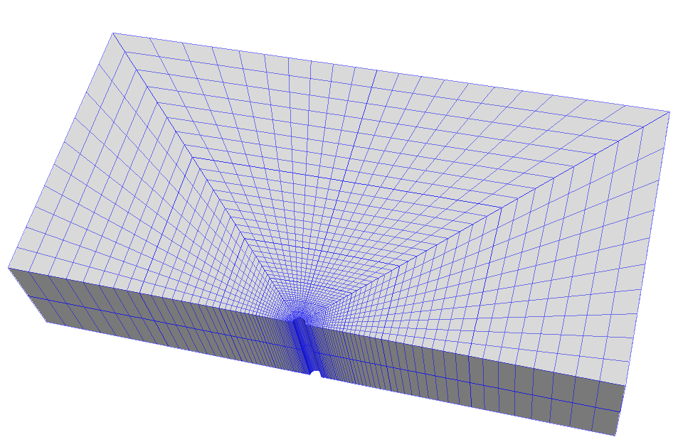
Fig. 50 Generated mesh for a vertical wellbore problem
Let us take a closer look at the geometry of this wellbore problem.
We use the internal wellbore mesh generator InternalWellbore to create a rock domain
( ), with a wellbore of
initial radius equal to
), with a wellbore of
initial radius equal to  m.
Coordinates of
m.
Coordinates of trajectory defines the wellbore trajectory, which represents a vertical well in this example.
By turning on autoSpaceRadialElems="{ 1 }", the internal mesh generator automatically sets number and spacing of elements in the radial direction, which overrides the values of nr.
With useCartesianOuterBoundary="0", a Cartesian aligned outer boundary on the outer block is enforced.
In this way, a structured three-dimensional mesh is created with 50 x 40 x 2 elements in the radial, tangential and z directions, respectively. All the elements are eight-node hexahedral elements (C3D8) and refinement is performed
to conform with the wellbore geometry. This mesh is defined as a cell block with the name
cb1.
  <Mesh>
    <InternalWellbore
      name="mesh1"
      elementTypes="{ C3D8 }"
      radius="{ 0.1, 5.0 }"
      theta="{ 0, 180 }"
      zCoords="{ -1, 1 }"
      nr="{ 40 }"
      nt="{ 40 }"
      nz="{ 2 }"
      trajectory="{ { 0.0, 0.0, -1.0 },
                    { 0.0, 0.0, 1.0 } }"
      autoSpaceRadialElems="{ 1 }"
      useCartesianOuterBoundary="0"
      cellBlockNames="{ cb1 }"/>
  </Mesh>
Solid mechanics solver
For the drained wellbore problem, the pore pressure variation is omitted. Therefore, we just need to define a solid mechanics solver, which is called mechanicsSolver.
This solid mechanics solver (see Solid Mechanics Solver) is based on the Lagrangian finite element formulation.
The problem is run as QuasiStatic without considering inertial effects.
The computational domain is discretized by FE1, which is defined in the NumericalMethods section.
The material is named as rock, whose mechanical properties are specified in the Constitutive section.
  <Solvers
    gravityVector="{ 0.0, 0.0, 0.0 }">
    <SolidMechanicsLagrangianFEM
      name="mechanicsSolver"
      logLevel="1"
      discretization="FE1"
      targetRegions="{ Omega }"
      >
      <LinearSolverParameters
      directParallel="0"/>
      <NonlinearSolverParameters
        newtonTol="1.0e-5"
        newtonMaxIter="15"/>
    </SolidMechanicsLagrangianFEM>
  </Solvers>
Constitutive laws
For this drained wellbore problem, we simulate the elastoplastic deformation caused by wellbore expansion.
A homogeneous domain with one solid material is assumed, whose mechanical properties are specified in the Constitutive section:
  <Constitutive>
    <ModifiedCamClay
      name="rock"
      defaultDensity="2700"
      defaultRefPressure="-1.2e5"
      defaultRefStrainVol="-0.0"
      defaultShearModulus="4.302e6"
      defaultPreConsolidationPressure="-1.69e5"
      defaultCslSlope="1.2"
      defaultVirginCompressionIndex="0.072676"
      defaultRecompressionIndex="0.014535"
    />
  </Constitutive>
Recall that in the SolidMechanicsLagrangianFEM section,
rock is designated as the material in the computational domain.
Here, Modified Cam-Clay ModifiedCamClay is used to simulate the elastoplastic behavior of rock.
The following material parameters should be defined properly to reproduce the analytical example:
XML Element: ModifiedCamClay
Name |
Type |
Default |
Description |
|---|---|---|---|
defaultCslSlope |
real64 |
1 |
Slope of the critical state line |
defaultDensity |
real64 |
required |
Default Material Density |
defaultDrainedLinearTEC |
real64 |
0 |
Default Linear Thermal Expansion Coefficient of the Solid Rock Frame |
defaultPreConsolidationPressure |
real64 |
-1.5 |
Initial preconsolidation pressure |
defaultRecompressionIndex |
real64 |
0.002 |
Recompresion Index |
defaultRefPressure |
real64 |
-1 |
Reference Pressure |
defaultRefStrainVol |
real64 |
0 |
Reference Volumetric Strain |
defaultShearModulus |
real64 |
-1 |
Elastic Shear Modulus Parameter |
defaultVirginCompressionIndex |
real64 |
0.005 |
Virgin compression index |
name |
groupName |
required |
A name is required for any non-unique nodes |
The constitutive parameters such as the density, the bulk modulus, and the shear modulus are specified in the International System of Units.
Initial and boundary conditions
The next step is to specify fields, including:
The initial value (the in-situ stresses and traction at the wellbore wall have to be initialized)
The boundary conditions (the reduction of wellbore pressure and constraints of the outer boundaries have to be set)
In this tutorial, we need to specify isotropic horizontal stress ( = -100 kPa) and vertical stress ( = -160 kPa).
To reach equilibrium, a compressive traction = -100 kPa is instantaneously applied at the wellbore wall rneg at time  = 0 s, which will then be gradually increased to a higher value (-300 kPa) to let wellbore expand.
The remaining parts of the outer boundaries are subjected to roller constraints.
These boundary conditions are set up through the
= 0 s, which will then be gradually increased to a higher value (-300 kPa) to let wellbore expand.
The remaining parts of the outer boundaries are subjected to roller constraints.
These boundary conditions are set up through the FieldSpecifications section.
  <FieldSpecifications>
    <FieldSpecification
      name="stressXX"
      initialCondition="1"
      setNames="{ all }"
      objectPath="ElementRegions"
      fieldName="rock_stress"
      component="0"
      scale="-1.0e5"/>

    <FieldSpecification
      name="stressYY"
      initialCondition="1"
      setNames="{ all }"
      objectPath="ElementRegions"
      fieldName="rock_stress"
      component="1"
      scale="-1.0e5"/>

    <FieldSpecification
      name="stressZZ"
      initialCondition="1"
      setNames="{ all }"
      objectPath="ElementRegions"
      fieldName="rock_stress"
      component="2"
      scale="-1.6e5"/>

    <Traction
      name="ExternalLoad"
      setNames="{ rneg }"
      objectPath="faceManager"
      scale="-1.0e5"
      tractionType="normal"
      functionName="timeFunction"/>

    <FieldSpecification
      name="xconstraint"
      objectPath="nodeManager"
      fieldName="totalDisplacement"
      component="0"
      scale="0.0"
      setNames="{ xneg, xpos }"/>

    <FieldSpecification
      name="yconstraint"
      objectPath="nodeManager"
      fieldName="totalDisplacement"
      component="1"
      scale="0.0"
      setNames="{ tneg, tpos, ypos }"/>

    <FieldSpecification
      name="zconstraint"
      objectPath="nodeManager"
      fieldName="totalDisplacement"
      component="2"
      scale="0.0"
      setNames="{ zneg, zpos }"/>
  </FieldSpecifications>
With tractionType="normal", traction is applied to the wellbore wall rneg as a pressure specified from the product of scale scale="-1.0e5" and the outward face normal.
A table function timeFunction is used to define the time-dependent traction ExternalLoad.
The coordinates and values form a time-magnitude
pair for the loading time history. In this case, the loading magnitude increases linearly as the time evolves.
  <Functions>
    <TableFunction
      name="timeFunction"
      inputVarNames="{ time }"
      coordinates="{ 0.0, 1.0 }"
      values="{ 1.0, 3.0 }"/>
  </Functions>
You may note :
All initial value fields must have
initialConditionfield set to1;The
setNamefield points to the previously defined set to apply the fields;
nodeManagerandfaceManagerin theobjectPathindicate that the boundary conditions are applied to the element nodes and faces, respectively;
fieldNameis the name of the field registered in GEOS;Component
0,1, and2refer to the x, y, and z direction, respectively;And the non-zero values given by
scaleindicate the magnitude of the loading;Some shorthand, such as
xnegandxpos, are used as the locations where the boundary conditions are applied in the computational domain. For instance,xnegmeans the face of the computational domain located at the left-most extent in the x-axis, whilexposrefers to the face located at the right-most extent in the x-axis. Similar shorthands includeypos,yneg,zpos, andzneg;The mud pressure loading has a negative value due to the negative sign convention for compressive stress in GEOS.
The parameters used in the simulation are summarized in the following table.
Symbol |
Parameter |
Units |
Value |
|---|---|---|---|
|
Reference Pressure |
[kPa] |
120 |
|
Shear Modulus |
[kPa] |
4302 |
|
PreConsolidation Pressure |
[kPa] |
169 |
|
Slope of CSL |
[-] |
1.2 |
|
Virgin Compression Index |
[-] |
0.072676 |
|
Recompression Index |
[-] |
0.014535 |
|
Horizontal Stress |
[kPa] |
-100 |
|
Vertical Stress |
[kPa] |
-160 |
|
Initial Well Radius |
[m] |
0.1 |
|
Mud Pressure |
[kPa] |
-300 |


Inspecting results
In the above example, we requested silo-format output files. We can therefore import these into VisIt and use python scripts to visualize the outcome. The following figure shows the distribution of  in the near wellbore region.
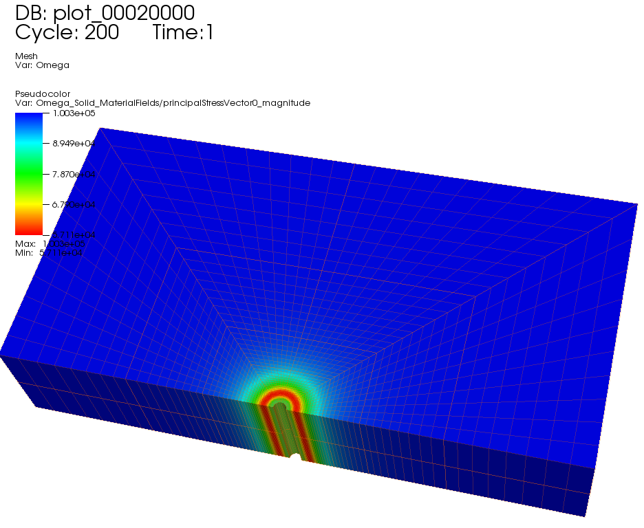
Fig. 51 Simulation result of
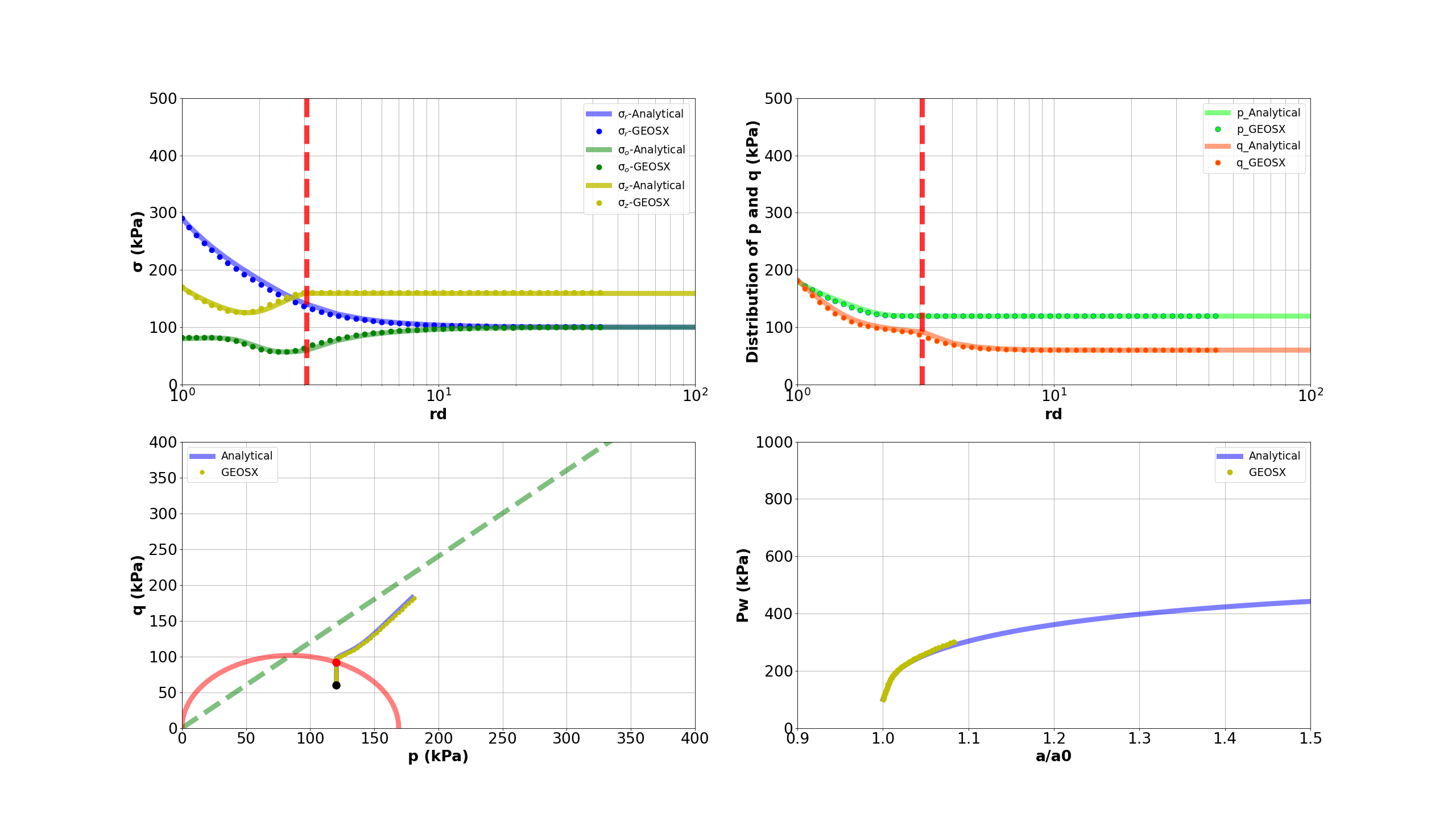
The figure below shows the comparisons between the numerical predictions (marks) and the corresponding analytical solutions (solid curves) with respect to the distributions of normal stress components, stress path, the supporting wellbore pressure and wellbore size. It is evident that the predictions well match the analytical results.
To go further
Feedback on this example
For any feedback on this example, please submit a GitHub issue on the project’s GitHub page.