Extended Drucker-Prager Model for Wellbore Problems
Context
The main goal of this example is to learn how to use the internal wellbore mesh generator and an elasto-plastic model to handle wellbore problems in GEOS. The Extended Drucker-Prager model (see Model: Extended Drucker-Prager) is applied to solve for elastoplastic deformation within the vicinity of a vertical wellbore. For the presented example, an analytical solution is employed to verify the accuracy of the numerical results. The resulting model can be used as a base for more complex analysis (e.g., wellbore drilling, fluid injection and storage scenarios).
Objectives
At the end of this example you will know:
how to construct meshes for wellbore problems with the internal mesh generator,
how to specify initial and boundary conditions, such as in-situ stresses and variation of traction at the wellbore wall,
how to use a plastic model for mechanical problems in the near wellbore region.
Input file
This example uses no external input files and everything required is contained within two xml files that are located at:
inputFiles/solidMechanics/ExtendedDruckerPragerWellbore_base.xml
inputFiles/solidMechanics/ExtendedDruckerPragerWellbore_benchmark.xml
The Python scripts for post-processing GEOS results, analytical restuls and validation plots are also provided in this example.
Description of the case
We simulate a drained wellbore problem subjected to isotropic horizontal stress ( ) and vertical stress (
 ). By lowering the wellbore supporting pressure (
 ), the wellbore contracts, and the reservoir rock experiences elastoplastic deformation. A plastic zone develops in the near wellbore region, as shown below.
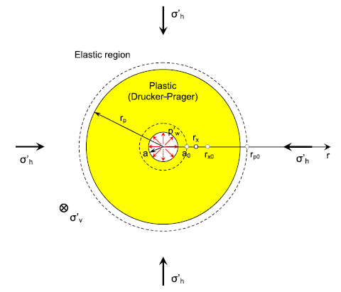
Fig. 45 Sketch of the wellbore problem (Chen and Abousleiman, 2017)
To simulate this phenomenon, the strain hardening Extended Drucker-Prager model with an associated plastic flow rule in GEOS is used in this example. Displacement and stress fields around the wellbore are numerically calculated. These numerical predictions are then compared with the corresponding analytical solutions (Chen and Abousleiman, 2017) from the literature.
All inputs for this case are contained inside a single XML file.
In this example, we focus our attention on the Mesh tags,
the Constitutive tags, and the FieldSpecifications tags.
Mesh
Following figure shows the generated mesh that is used for solving this 3D wellbore problem
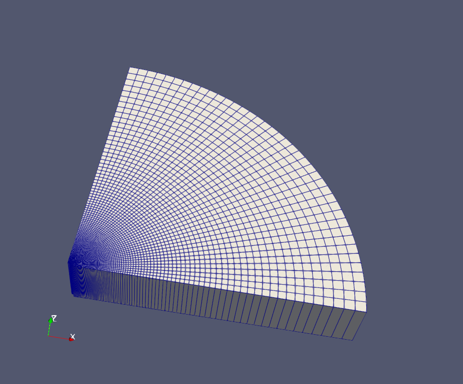
Fig. 46 Generated mesh for the wellbore problem
Let us take a closer look at the geometry of this wellbore problem.
We use the internal mesh generator InternalWellbore to create a rock domain
( ), with a wellbore of
initial radius equal to
), with a wellbore of
initial radius equal to  m.
Coordinates of
m.
Coordinates of trajectory defines the wellbore trajectory, which represents a vertical well in this example.
By turning on autoSpaceRadialElems="{ 1 }", the internal mesh generator automatically sets number and spacing of elements in the radial direction, which overrides the values of nr. In this way, a structured three-dimensional mesh is created. All the elements are eight-node hexahedral elements (C3D8) and refinement is performed
to conform with the wellbore geometry. This mesh is defined as a cell block with the name
cb1.
  <Mesh>
    <InternalWellbore
      name="mesh1"
      elementTypes="{ C3D8 }"
      radius="{ 0.1, 10.0 }"
      theta="{ 0, 90 }"
      zCoords="{ -1, 1 }"
      nr="{ 40 }"
      nt="{ 40 }"
      nz="{ 1 }"
      trajectory="{ { 0.0, 0.0, -1.0 },
                    { 0.0, 0.0, 1.0 } }"
      autoSpaceRadialElems="{ 1 }"
      cellBlockNames="{ cb1 }"/>
  </Mesh>
Solid mechanics solver
For the drained wellbore problem, the pore pressure variation is omitted and can be subtracted from the analysis. Therefore, we just need to define a solid mechanics solver, which is called mechanicsSolver.
This solid mechanics solver (see Solid Mechanics Solver) is based on the Lagrangian finite element formulation.
The problem is run as QuasiStatic without considering inertial effects.
The computational domain is discretized by FE1, which is defined in the NumericalMethods section.
The material is named as rock, whose mechanical properties are specified in the Constitutive section.
  <Solvers
    gravityVector="{ 0.0, 0.0, 0.0 }">
    <SolidMechanicsLagrangianFEM
      name="mechanicsSolver"
      logLevel="1"
      discretization="FE1"
      targetRegions="{ Omega }"
      >
      <LinearSolverParameters
        directParallel="0"/>
      <NonlinearSolverParameters
        newtonTol="1.0e-5"
        newtonMaxIter="15"/>
    </SolidMechanicsLagrangianFEM>
  </Solvers>
Constitutive laws
For this drained wellbore problem, we simulate the elastoplastic deformation caused by wellbore contraction.
A homogeneous domain with one solid material is assumed, whose mechanical properties are specified in the Constitutive section:
  <Constitutive>
    <ExtendedDruckerPrager
      name="rock"
      defaultDensity="2700"
      defaultBulkModulus="0.5e9"
      defaultShearModulus="0.3e9"
      defaultCohesion="0.0"
      defaultInitialFrictionAngle="15.27"
      defaultResidualFrictionAngle="23.05"
      defaultDilationRatio="1.0"
      defaultHardening="0.01"/>

  </Constitutive>
Recall that in the SolidMechanicsLagrangianFEM section,
rock is designated as the material in the computational domain.
Here, Extended Drucker Prager model ExtendedDruckerPrager is used to simulate the elastoplastic behavior of rock.
As for the material parameters, defaultInitialFrictionAngle, defaultResidualFrictionAngle and defaultCohesion denote the initial friction angle, the residual friction angle, and cohesion, respectively, as defined by the Mohr-Coulomb failure envelope. In this example, zero cohesion is considered to consist with the reference analytical results. As the residual friction angle defaultResidualFrictionAngle is larger than the initial one defaultInitialFrictionAngle, a strain hardening model is adopted, whose hardening rate is given as defaultHardening="0.01".
If the residual friction angle is set to be less than the initial one, strain weakening will take place.
Setting defaultDilationRatio="1.0" corresponds to an associated flow rule.
The constitutive parameters such as the density, the bulk modulus, and the shear modulus are specified in the International System of Units.
Initial and boundary conditions
The next step is to specify fields, including:
The initial value (the in-situ stresses and traction at the wellbore wall have to be initialized)
The boundary conditions (the reduction of wellbore pressure and constraints of the outer boundaries have to be set)
In this example, we need to specify isotropic horizontal stress ( = -11.25 MPa) and vertical stress ( = -15.0 MPa).
To reach equilibrium, a compressive traction  = -11.25 MPa is instantaneously applied at the wellbore wall
 rneg at time  = 0 s, which will then be gradually reduced to a lower absolute value (-2.0 MPa) to let wellbore contract.
The boundaries at
= 0 s, which will then be gradually reduced to a lower absolute value (-2.0 MPa) to let wellbore contract.
The boundaries at tneg and tpos are subjected to roller constraints. The plane strain condition is ensured by fixing the vertical displacement at zneg and zpos The far-field boundary is fixed in horizontal displacement.
These boundary conditions are set up through the FieldSpecifications section.
  <FieldSpecifications>
    <FieldSpecification
      name="stressXX"
      initialCondition="1"
      setNames="{ all }"
      objectPath="ElementRegions/Omega/cb1"
      fieldName="rock_stress"
      component="0"
      scale="-11.25e6"/>

    <FieldSpecification
      name="stressYY"
      initialCondition="1"
      setNames="{ all }"
      objectPath="ElementRegions/Omega/cb1"
      fieldName="rock_stress"
      component="1"
      scale="-11.25e6"/>

    <FieldSpecification
      name="stressZZ"
      initialCondition="1"
      setNames="{ all }"
      objectPath="ElementRegions/Omega/cb1"
      fieldName="rock_stress"
      component="2"
      scale="-15.0e6"/>

    <Traction
      name="ExternalLoad"
      setNames="{ rneg }"
      objectPath="faceManager"
      scale="1.0"
      tractionType="normal"
      functionName="timeFunction"/>

    <FieldSpecification
      name="xconstraint"
      objectPath="nodeManager"
      fieldName="totalDisplacement"
      component="0"
      scale="0.0"
      setNames="{ tpos, rpos }"/>

    <FieldSpecification
      name="yconstraint"
      objectPath="nodeManager"
      fieldName="totalDisplacement"
      component="1"
      scale="0.0"
      setNames="{ tneg, rpos }"/>

    <FieldSpecification
      name="zconstraint"
      objectPath="nodeManager"
      fieldName="totalDisplacement"
      component="2"
      scale="0.0"
      setNames="{ zneg, zpos }"/>
  </FieldSpecifications>
With tractionType="normal", traction is applied to the wellbore wall rneg as a pressure specified from the product of scale scale="1.0" and the outward face normal.
A table function timeFunction is used to define the time-dependent traction ExternalLoad.
The coordinates and values form a time-magnitude
pair for the loading time history. In this case, the loading magnitude decreases linearly as the time evolves.
  <Functions>
    <TableFunction
      name="timeFunction"
      inputVarNames="{ time }"
      coordinates="{ 0.0, 1.0, 1e99 }"
      values="{ -11.25e6, -2.0e6, -2.0e6 }"/>
  </Functions>
You may note :
All initial value fields must have
initialConditionfield set to1;The
setNamefield points to the previously defined box to apply the fields;
nodeManagerandfaceManagerin theobjectPathindicate that the boundary conditions are applied to the element nodes and faces, respectively;
fieldNameis the name of the field registered in GEOS;Component
0,1, and2refer to the x, y, and z direction, respectively;And the non-zero values given by
Scaleindicate the magnitude of the loading;Some shorthand, such as
tposandxpos, are used as the locations where the boundary conditions are applied in the computational domain. For instance,tposmeans the portion of the computational domain located at the left-most in the x-axis, whilexposrefers to the portion located at the right-most area in the x-axis. Similar shorthand includeypos,tneg,zpos, andzneg;The mud pressure loading has a negative value due to the negative sign convention for compressive stress in GEOS.
The parameters used in the simulation are summarized in the following table.
Symbol |
Parameter |
Unit |
Value |
|---|---|---|---|
|
Bulk modulus |
[MPa] |
500 |
|
Shear Modulus |
[MPa] |
300 |
|
Cohesion |
[MPa] |
0.0 |
|
Initial Friction Angle |
[degree] |
15.27 |
|
Residual Friction Angle |
[degree] |
23.05 |
|
Hardening Rate |
[-] |
0.01 |
|
Horizontal Stress |
[MPa] |
-11.25 |
|
Vertical Stress |
[MPa] |
-15.0 |
|
Initial Well Radius |
[m] |
0.1 |
|
Mud Pressure |
[MPa] |
-2.0 |


Inspecting results
In the above example, we requested hdf5 output files. We can therefore use python scripts to visualize the outcome. Below figure shows the comparisons between the numerical predictions (marks) and the corresponding analytical solutions (solid curves) with respect to the distributions of principal stress components, stress path on the wellbore surface, the supporting wellbore pressure and wellbore size. It is clear that the GEOS predictions are in excellent agreement with the analytical results. On the top-right figure, we added also a comparison between GEOS results for elasto-plastic material and the anlytical solutions of an elastic material. Note that the elastic solutions are differed from the elasto-plastic results even in the elastic zone (r/a>2).
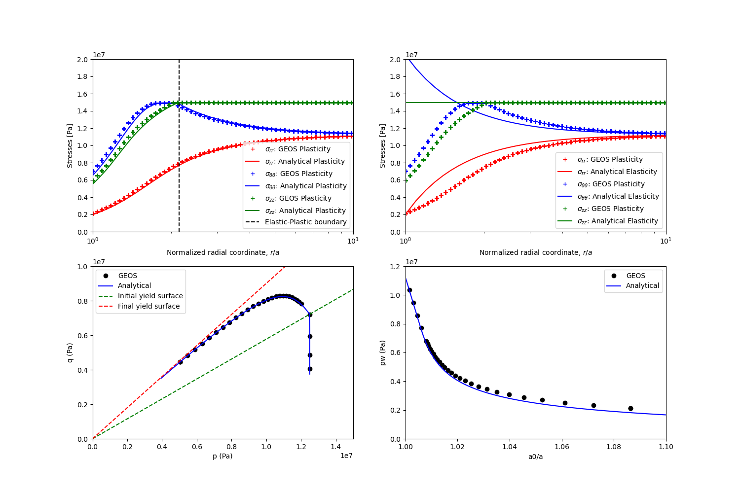
Fig. 47 Validation of GEOS results.
For the same wellbore problem, using different constitutive models (plastic vs. elastic), obviously, distinct differences in rock deformation and distribution of resultant stresses is also observed and highlighted.
To go further
Feedback on this example
This concludes the example on Plasticity Model for Wellbore Problems. For any feedback on this example, please submit a GitHub issue on the project’s GitHub page.
For more details
More on plasticity models, please see Model: Extended Drucker-Prager.
More on functions, please see Functions.