Fracture Intersection Problem
Context
In this example, two fractures intersecting at a right angle are simulated using a Lagrange contact model in a 2D infinite domain and subjected to a constant uniaxial compressive remote stress. Numerical solutions based on the symmetric-Galerkin boundary element
method (Phan et al., 2003) is used to verify the accuracy of the GEOS results for the normal traction, normal opening, and shear slippage on the fracture surfaces, considering frictional contact and fracture-fracture interaction. In this example, the TimeHistory function and a Python script are used to output and post-process multi-dimensional data (traction and displacement on the fracture surfaces).
Input file
Everything required is contained within these xml files located at:
inputFiles/lagrangianContactMechanics/TFrac_base.xml
inputFiles/lagrangianContactMechanics/TFrac_benchmark.xml
inputFiles/lagrangianContactMechanics/ContactMechanics_TFrac_benchmark.xml
Description of the case
We simulate two intersecting fractures under a remote compressive stress constraint, as shown below. The two fractures sit in an infinite, homogeneous, isotropic, and elastic medium. The vertical fracture is internally pressurized and perpendicularly intersects the middle of the horizontal fracture. A combination of uniaxial compression, frictional contact, and opening of the vertical fracture causes mechanical deformations of the surrounding rock, thus leads to sliding of the horizontal fracture. For verification purposes, a plane strain deformation and Coulomb failure criterion are considered in this numerical model.
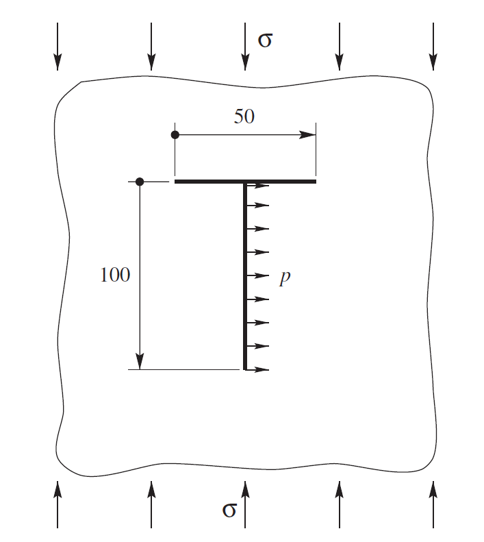
Fig. 23 Sketch of the problem (Phan et al., 2003)
To simulate this problem, we use a Lagrange contact model. Displacement and stress fields on the fracture plane are calculated numerically. Predictions of the normal traction and slip along the sliding fracture and mechanical aperture of the pressurized fracture are compared with the corresponding literature work (Phan et al., 2003).
For this example, we focus on the Mesh,
the Constitutive, and the FieldSpecifications tags.
Mesh
The following figure shows the mesh used in this problem.
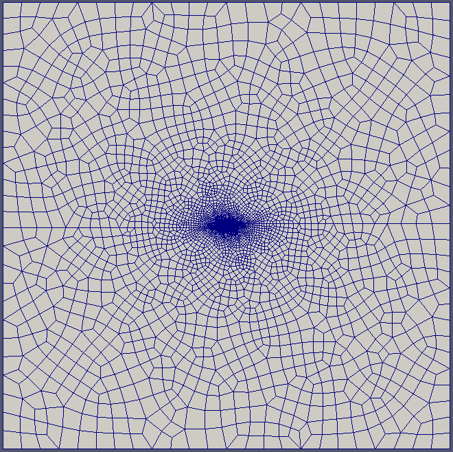
Fig. 24 Generated mesh
This mesh was created using the internal mesh generator as parametrized in the InternalMesh XML tag.
The mesh contains 300 x 300 x 2 eight-node brick elements in the x, y, and z directions respectively.
Such eight-node hexahedral elements are defined as C3D8 elementTypes, and their collection forms a mesh
with one group of cell blocks named here cb1.
  <Mesh>
    <InternalMesh
      name="mesh1"
      elementTypes="{ C3D8 }"
      xCoords="{ -1000, -100, 100, 1000 }"
      yCoords="{ -1000, -100, 100, 1000 }"
      zCoords="{ 0, 2 }"
      nx="{ 150, 200, 150 }"
      ny="{ 150, 200, 150 }"
      nz="{ 2 }"
      cellBlockNames="{ cb1 }"/>
  </Mesh>
Refinement is necessary to conform with the fracture geometry specified in the Geometry section.
  <Geometry>
    <Rectangle
      name="fracture1"
      normal="{1.0, 0.0, 0.0}"
      origin="{0.0, 0.0, 0.0}"
      lengthVector="{0.0, 1.0, 0.0}"
      widthVector="{0.0, 0.0, 1.0}"
      dimensions="{ 100, 200 }"/>

    <Rectangle
      name="core1"
      normal="{1.0, 0.0, 0.0}"
      origin="{0.0, 0.0, 0.0}"
      lengthVector="{0.0, 1.0, 0.0}"
      widthVector="{0.0, 0.0, 1.0}"
      dimensions="{ 100, 200 }"/>

    <Rectangle
      name="fracture2"
      normal="{0.0, 1.0, 0.0}"
      origin="{0.0, 50.0, 0.0}"
      lengthVector="{1.0, 0.0, 0.0}"
      widthVector="{0.0, 0.0, 1.0}"
      dimensions="{ 50, 200 }"/>

    <Rectangle
      name="core2"
      normal="{0.0, 1.0, 0.0}"
      origin="{0.0, 50.0, 0.0}"
      lengthVector="{1.0, 0.0, 0.0}"
      widthVector="{0.0, 0.0, 1.0}"
      dimensions="{ 50, 200 }"/>
  </Geometry>
Solid mechanics solver
GEOS is a multiphysics simulation platform.
Different combinations of
physics solvers can be applied
in different regions of the domain at different stages of the simulation.
The Solvers tag in the XML file is used to list and parameterize these solvers.
To specify a coupling between two different solvers, we define and characterize each single-physics solver separately. Then, we customize a coupling solver between these single-physics solvers as an additional solver. This approach allows for generality and flexibility in constructing multiphysics solvers. Each single-physics solver should be given a meaningful and distinct name, because GEOS recognizes these single-physics solvers by their given names to create the coupling.
To setup a coupling between rock and fracture deformations, we define three different solvers:
For solving the frictional contact, we define a Lagrangian contact solver, called here
lagrangiancontact. In this solver, we specifytargetRegionsthat include both the continuum regionRegionand the discontinuum regionFracturewhere the solver is applied to couple rock and fracture deformations. The contact constitutive law used for the fracture elements is namedfractureMaterial, and is defined later in theConstitutivesection.Rock deformations are handled by a solid mechanics solver
SolidMechanicsLagrangianFEM. This solid mechanics solver (see SolidMechanicsLagrangianFEM) is based on the Lagrangian finite element formulation. The problem runs inQuasiStaticmode without inertial effects. The computational domain is discretized byFE1, which is defined in theNumericalMethodssection. The solid material is namedrockand its mechanical properties are specified later in theConstitutivesection.The solver
SurfaceGeneratordefines the fracture region and rock toughness.
  <SolidMechanicsLagrangeContact
   name="lagrangiancontact"
   stabilizationName="TPFAstabilization"
   logLevel="1"
   discretization="FE1"
   targetRegions="{ Region, Fracture }">
   <NonlinearSolverParameters
     newtonTol="1.0e-5"
     logLevel="2"
     maxNumConfigurationAttempts="10"
     newtonMaxIter="10"
     lineSearchAction="Require"
     lineSearchMaxCuts="2"
     maxTimeStepCuts="2"/>
   <LinearSolverParameters
     solverType="gmres"
     preconditionerType="mgr"
     krylovTol="1e-8"
     logLevel="0"/>
  </SolidMechanicsLagrangeContact>
Constitutive laws
For this problem, we simulate the elastic deformation and fracture slippage caused by the uniaxial compression.
A homogeneous and isotropic domain with one solid material is assumed, and its mechanical properties are specified in the Constitutive section.
Fracture surface slippage is assumed to be governed by the Coulomb failure criterion. The contact constitutive behavior is named fractureMaterial in the Coulomb block, where cohesion cohesion="0.0" and friction coefficient frictionCoefficient="0.577350269" are specified.
  <Constitutive>
    <ElasticIsotropic
      name="rock"
      defaultDensity="2700"
      defaultBulkModulus="38.89e9"
      defaultShearModulus="29.17e9"/>

    <Coulomb
      name="frictionLaw"
      defaultCohesion="0.0"
      defaultFrictionCoefficient="0.577350269"/>
  </Constitutive>
Recall that in the SolidMechanicsLagrangianFEM section,
rock is the material of the computational domain.
Here, the isotropic elastic model ElasticIsotropic is used to simulate the mechanical behavior of rock.
All constitutive parameters such as density, bulk modulus, and shear modulus are specified in the International System of Units.
Time history function
In the Tasks section, PackCollection tasks are defined to collect time history information from fields.
Either the entire field or specified named sets of indices in the field can be collected.
In this example, tractionCollection and displacementJumpCollection tasks are specified to output the local traction fieldName="traction" and relative displacement fieldName="displacementJump" on the fracture surface.
  <Tasks>
    <PackCollection
      name="tractionCollection"
      objectPath="ElementRegions/Fracture/faceElementSubRegion"
      fieldName="traction"/>

    <PackCollection
      name="displacementJumpCollection"
      objectPath="ElementRegions/Fracture/faceElementSubRegion"
      fieldName="displacementJump"/>
  </Tasks>
These two tasks are triggered using the Event manager with a PeriodicEvent defined for these recurring tasks.
GEOS writes two files named after the string defined in the filename keyword and formatted as HDF5 files (displacementJump_history.hdf5 and traction_history.hdf5). The TimeHistory file contains the collected time history information from each specified time history collector.
This information includes datasets for the simulation time, element center defined in the local coordinate system, and the time history information.
A Python script is used to read and plot any specified subset of the time history data for verification and visualization.
Initial and boundary conditions
The next step is to specify fields, including:
The initial value (the remote compressive stress needs to be initialized),
The boundary conditions (traction loaded on the vertical fracture and the constraints of the outer boundaries have to be set).
In this tutorial, we specify an uniaxial vertical stress SigmaY ( = -1.0e8 Pa).
A compressive traction
= -1.0e8 Pa).
A compressive traction NormalTraction ( = -1.0e8 Pa) is applied at the surface of vertical fracture.
The remaining parts of the outer boundaries are subjected to roller constraints.
These boundary conditions are set up through the
= -1.0e8 Pa) is applied at the surface of vertical fracture.
The remaining parts of the outer boundaries are subjected to roller constraints.
These boundary conditions are set up through the FieldSpecifications section.
  <FieldSpecifications>
    <FieldSpecification
      name="frac"
      initialCondition="1"
      setNames="{ fracture1, fracture2 }"
      objectPath="faceManager"
      fieldName="ruptureState"
      scale="1"/>

    <FieldSpecification
      name="separableFace"
      initialCondition="1"
      setNames="{ core1, core2 }"
      objectPath="faceManager"
      fieldName="isFaceSeparable"
      scale="1"/>

    <FieldSpecification
      name="xconstraint"
      objectPath="nodeManager"
      fieldName="totalDisplacement"
      component="0"
      scale="0.0"
      setNames="{ xpos, xneg }"/>

    <FieldSpecification
      name="yconstraint"
      objectPath="nodeManager"
      fieldName="totalDisplacement"
      component="1"
      scale="0.0"
      setNames="{ ypos, yneg }"/>

    <FieldSpecification
      name="zconstraint"
      objectPath="nodeManager"
      fieldName="totalDisplacement"
      component="2"
      scale="0.0"
      setNames="{ zpos, zneg }"/>

    <Traction
      name="NormalTraction"
      objectPath="faceManager"
      tractionType="normal"
      scale="-1.0e8"
      functionName="ForceTimeFunction"
      setNames="{ core1 }"/>

    <FieldSpecification
      name="SigmaY"
      initialCondition="1"
      setNames="{ all }"
      objectPath="ElementRegions/Region"
      fieldName="rock_stress"
      component="1"
      scale="-1.0e8"/>
  </FieldSpecifications>
Note that the remote stress and internal fracture pressure has a negative value, due to the negative sign convention for compressive stresses in GEOS.
The parameters used in the simulation are summarized in the following table.
Symbol |
Parameter |
Unit |
Value |
|---|---|---|---|
|
Bulk Modulus |
[GPa] |
38.89 |
|
Shear Modulus |
[GPa] |
29.17 |
|
Remote Stress |
[MPa] |
-100.0 |
|
Internal Pressure |
[MPa] |
-100.0 |
|
Friction Angle |
[Degree] |
30.0 |
|
Horizontal Frac Length |
[m] |
50.0 |
|
Vertical Frac Length |
[m] |
100.0 |


Inspecting results
We request VTK-format output files and use Paraview to visualize the results.
The following figure shows the distribution of  in the computational domain.
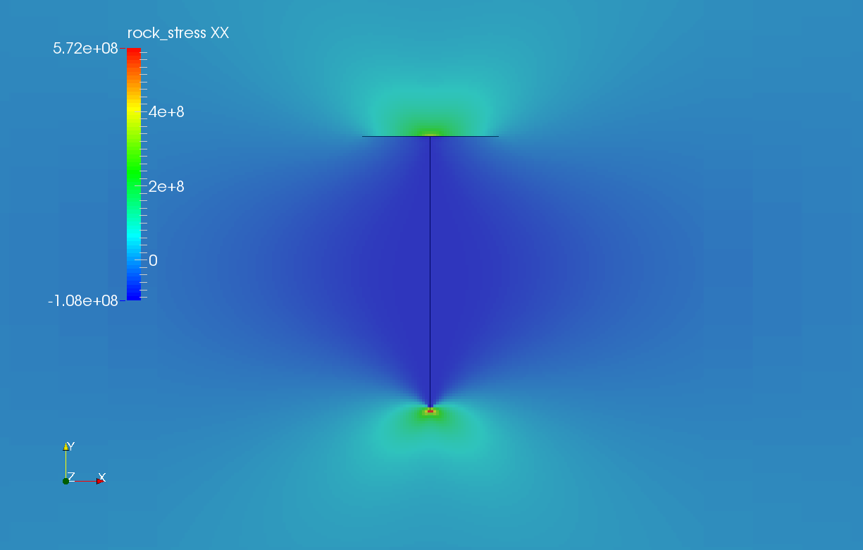
Fig. 25 Simulation result of
The next figure shows the distribution of relative shear displacement values along the surface of two intersected fractures.
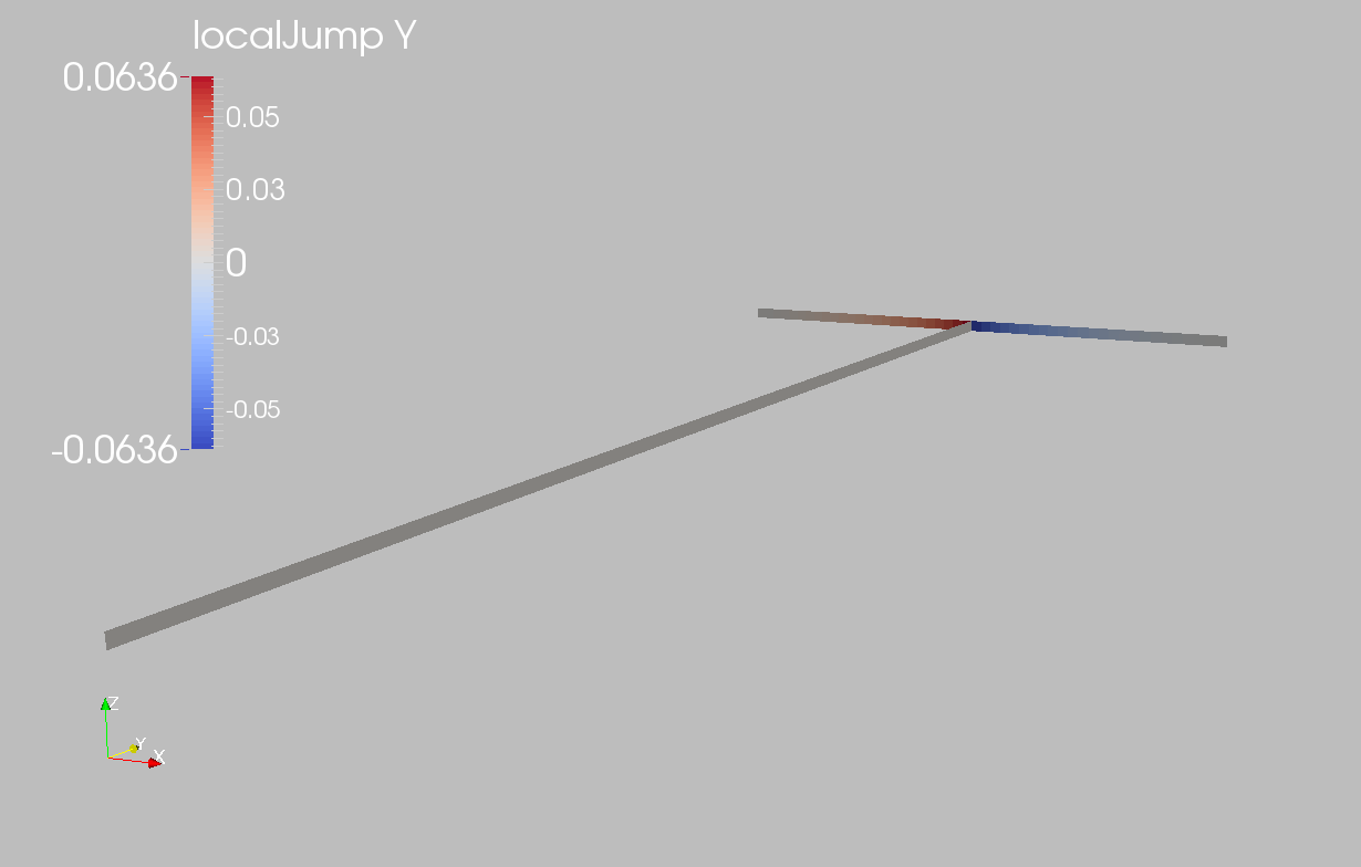
Fig. 26 Simulation result of fracture slip
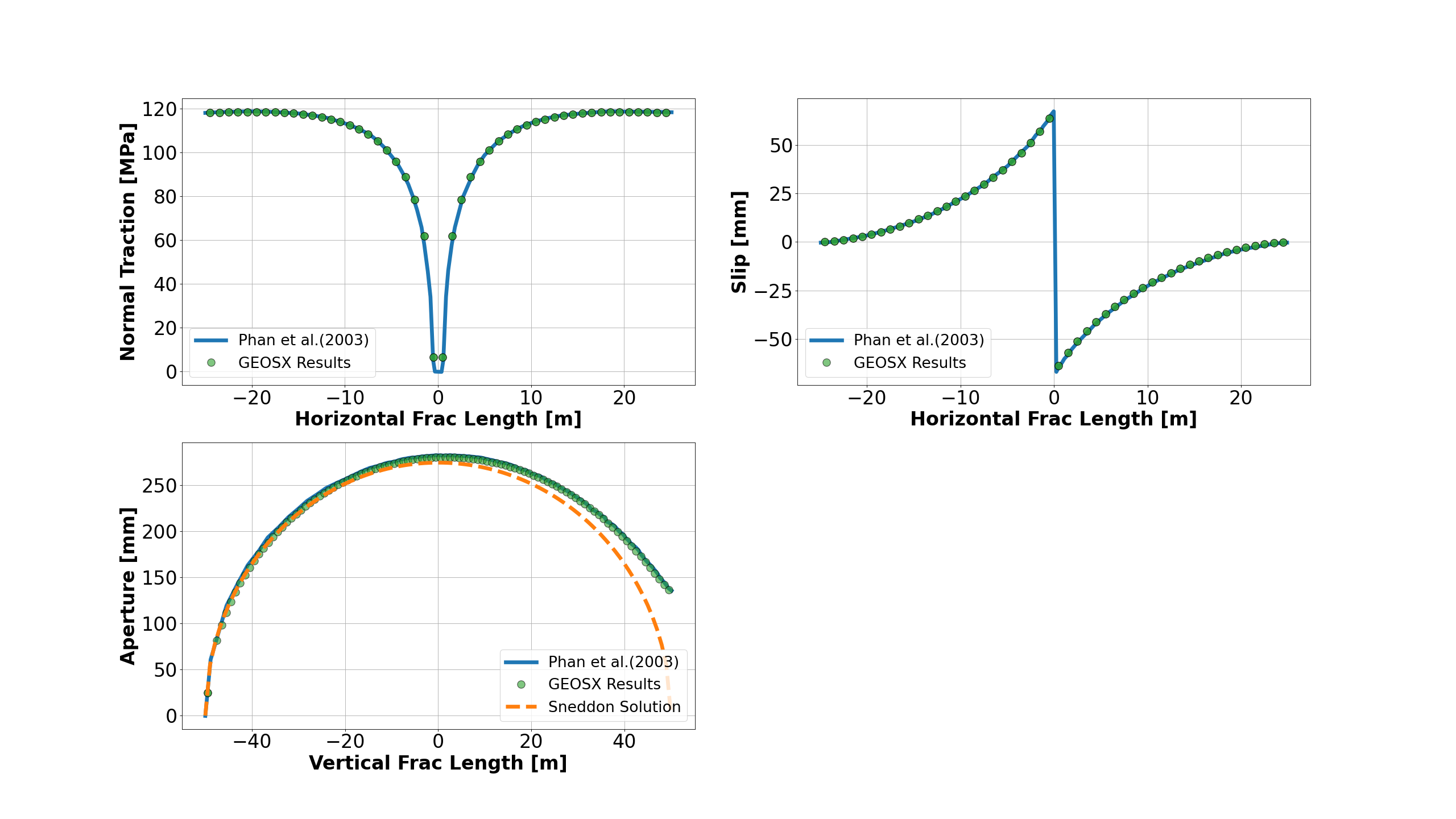
The figure below compares the results from GEOS (marks) and the corresponding literature reference solution (solid curves) for the normal traction and slip distributions along the horizontal fracture and opening of the vertical fracture. GEOS reliably captures the mechanical interactions between two intersected fractures and shows excellent agreement with the reference solution. Due to sliding of the horizontal fracture, GEOS prediction as well as the reference solution on the normal opening of pressurized vertical fracture deviates away from Sneddon’s analytical solution, especially near the intersection point.
To go further
Feedback on this example
For any feedback on this example, please submit a GitHub issue on the project’s GitHub page.