Poromechanics

Context

In this example, we use a coupled solver to solve a poroelastic Terzaghi-type problem, a classic benchmark in poroelasticity. We do so by coupling a single phase flow solver with a small-strain Lagrangian mechanics solver.

Objectives

At the end of this example you will know:

how to use multiple solvers for poromechanical problems,

how to define finite elements and finite volume numerical methods.

Input file

This example uses no external input files and everything required is contained within two GEOS input files located at:

inputFiles/poromechanics/PoroElastic_Terzaghi_base_direct.xml

inputFiles/poromechanics/PoroElastic_Terzaghi_smoke.xml

Description of the case

We simulate the consolidation of a poroelastic fluid-saturated column of height $L$ having unit cross-section. The column is instantaneously loaded at time $t$ = 0 s with a constant compressive traction $w$ applied on the face highlighted in red in the figure below. Only the loaded face if permeable to fluid flow, with the remaining parts of the boundary subject to roller constraints and impervious.

../../../../_images/terzaghi_sketch.svg — Fig. 1 Sketch of the setup for Terzaghi’s problem.

GEOS will calculate displacement and pressure fields along the column as a function of time. We will use the analytical solution for pressure to check the accuracy of the solution obtained with GEOS, namely

$p(x,t) = \frac{4}{\pi} p_0 \sum_{m=0}^{\infty} \frac{1}{2m + 1} \text{exp} \left[ -\frac{(2m + 1)^2 \pi^2 c_c t}{4 L^2} \right] \text{sin} \left[ \frac{(2m+1)\pi x}{2L} \right],$

where $p_0 = \frac{b}{K_vS_{\epsilon} + b^2} |w|$ is the initial pressure, constant throughout the column, and $c_c = \frac{\kappa}{\mu} \frac{K_v}{K_v S_{\epsilon} + b^2}$ is the consolidation coefficient (or diffusion coefficient), with

$b$ Biot’s coefficient
$K_v = \frac{E(1-\nu)}{(1+\nu)(1-2\nu)}$ the uniaxial bulk modulus, $E$ Young’s modulus, and $\nu$ Poisson’s ratio
$S_{\epsilon}=\frac{(b - \phi)(1 - b)}{K} + \phi c_f$ the constrained specific storage coefficient, $\phi$ porosity, $K = \frac{E}{3(1-2\nu)}$ the bulk modulus, and $c_f$ the fluid compressibility
$\kappa$ the isotropic permeability
$\mu$ the fluid viscosity

The characteristic consolidation time of the system is defined as $t_c = \frac{L^2}{c_c}$ . Knowledge of $t_c$ is useful for choosing appropriately the timestep sizes that are used in the discrete model.

Coupled solvers

GEOS is a multi-physics tool. Different combinations of physics solvers available in the code can be applied in different regions of the mesh at different moments of the simulation. The XML Solvers tag is used to list and parameterize these solvers.

We define and characterize each single-physics solver separately. Then, we define a coupling solver between these single-physics solvers as another, separate, solver. This approach allows for generality and flexibility in our multi-physics resolutions. The order in which these solver specifications is done is not important. It is important, though, to instantiate each single-physics solver with meaningful names. The names given to these single-physics solver instances will be used to recognize them and create the coupling.

To define a poromechanical coupling, we will effectively define three solvers:

the single-physics flow solver, a solver of type SinglePhaseFVM called here SinglePhaseFlowSolver (more information on these solvers at Singlephase Flow Solver),

the small-stress Lagrangian mechanics solver, a solver of type SolidMechanicsLagrangianSSLE called here LinearElasticitySolver (more information here: Solid Mechanics Solver),

the coupling solver that will bind the two single-physics solvers above, an object of type SinglePhasePoromechanics called here PoroelasticitySolver (more information at Poromechanics Solver).

Note that the name attribute of these solvers is chosen by the user and is not imposed by GEOS.

The two single-physics solvers are parameterized as explained in their respective documentation.

Let us focus our attention on the coupling solver. This solver (PoroelasticitySolver) uses a set of attributes that specifically describe the coupling for a poromechanical framework. For instance, we must point this solver to the correct fluid solver (here: SinglePhaseFlowSolver), the correct solid solver (here: LinearElasticitySolver). Now that these two solvers are tied together inside the coupling solver, we have a coupled multiphysics problem defined. More parameters are required to characterize a coupling. Here, we specify the discretization method (FE1, defined further in the input file), and the target regions (here, we only have one, Domain).

    <SinglePhasePoromechanics
      name="PoroelasticitySolver"
      solidSolverName="LinearElasticitySolver"
      flowSolverName="SinglePhaseFlowSolver"
      logLevel="1"
      targetRegions="{ Domain }">
      <LinearSolverParameters
        directParallel="0"/>
    </SinglePhasePoromechanics>

    <SolidMechanicsLagrangianSSLE
      name="LinearElasticitySolver"
      timeIntegrationOption="QuasiStatic"
      logLevel="1"
      discretization="FE1"
      targetRegions="{ Domain }"/>

    <SinglePhaseFVM
      name="SinglePhaseFlowSolver"
      logLevel="1"
      discretization="singlePhaseTPFA"
      targetRegions="{ Domain }"/>
  </Solvers>

Multiphysics numerical methods

Numerical methods in multiphysics settings are similar to single physics numerical methods. All can be defined under the same NumericalMethods XML tag. In this problem, we use finite volume for flow and finite elements for solid mechanics. Both methods require additional parameterization attributes to be defined here.

As we have seen before, the coupling solver and the solid mechanics solver require the specification of a discretization method called FE1. This discretization method is defined here as a finite element method using linear basis functions and Gaussian quadrature rules. For more information on defining finite elements numerical schemes, please see the dedicated FiniteElement section.

The finite volume method requires the specification of a discretization scheme. Here, we use a two-point flux approximation as described in the dedicated documentation (found here: FiniteVolume).

  <NumericalMethods>
    <FiniteElements>
      <FiniteElementSpace
        name="FE1"
        order="1"/>
    </FiniteElements>

    <FiniteVolume>
      <TwoPointFluxApproximation
        name="singlePhaseTPFA"/>
    </FiniteVolume>
  </NumericalMethods>

Mesh, material properties, and boundary conditions

Last, let us take a closer look at the geometry of this simple problem. We use the internal mesh generator to create a beam-like mesh, with one single element along the Y and Z axes, and 21 elements along the X axis. All the elements are hexahedral elements (C3D8) of the same dimension (1x1x1 meters).

  <Mesh>
    <InternalMesh
      name="mesh1"
      elementTypes="{ C3D8 }"
      xCoords="{ 0, 10 }"
      yCoords="{ 0, 1 }"
      zCoords="{ 0, 1 }"
      nx="{ 400 }"
      ny="{ 16 }"
      nz="{ 16 }"
      cellBlockNames="{ cb1 }"/>
  </Mesh>

The parameters used in the simulation are summarized in the following table.

Symbol	Parameter	Units	Value
$E$	Young’s modulus	[Pa]	10⁴
$\nu$	Poisson’s ratio	[-]	0.2
$b$	Biot’s coefficient	[-]	1.0
$\phi$	Porosity	[-]	0.3
$\rho_f$	Fluid density	[kg/m³]	1.0
$c_f$	Fluid compressibility	[Pa^-1]	0.0
$\kappa$	Permeability	[m²]	10^-4
$\mu$	Fluid viscosity	[Pa s]	1.0
$\|w\|$	Applied compression	[Pa]	1.0
$L$	Column length	[m]	10.0

Material properties and boundary conditions are specified in the Constitutive and FieldSpecifications sections. For such set of parameters we have $p_0$ = 1.0 Pa, $c_c$ = 1.111 m² s^-1, and $t_c$ = 90 s. Therefore, as shown in the Events section, we run this simulation for 90 seconds.

Running GEOS

To run the case, use the following command:

path/to/geosx -i inputFiles/poromechanics/PoroElastic_Terzaghi_smoke.xml

Here, we see for instance the RSolid and RFluid at a representative timestep (residual values for solid and fluid mechanics solvers, respectively)

Attempt:  0, NewtonIter:  0
( RSolid ) = (5.00e-01) ;     ( Rsolid, Rfluid ) = ( 5.00e-01, 0.00e+00 )
( R ) = ( 5.00e-01 ) ;
Attempt:  0, NewtonIter:  1
( RSolid ) = (4.26e-16) ;     ( Rsolid, Rfluid ) = ( 4.26e-16, 4.22e-17 )
( R ) = ( 4.28e-16 ) ;

As expected, since we are dealing with a linear problem, the fully implicit solver converges in a single iteration.

Inspecting results

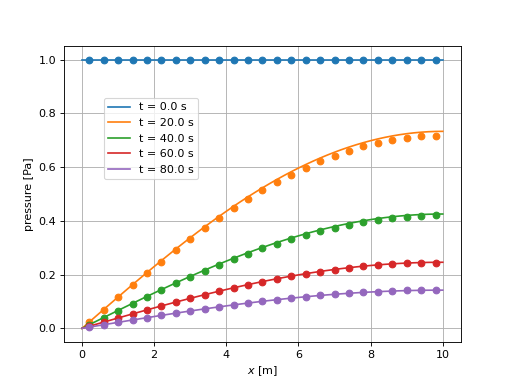
This plot compares the analytical pressure solution (continuous lines) at selected times with the numerical solution (markers).

(Source code)

../../../../_images/poromechanicsFigure.png

To go further

Feedback on this example

This concludes the poroelastic example. For any feedback on this example, please submit a GitHub issue on the project’s GitHub page.

For more details

More on poroelastic multiphysics solvers, please see Poromechanics Solver.

More on numerical methods, please see Numerical Methods.

More on functions, please see Functions.