Tutorial 6: CO 2 injection into an unstructured grid
Context
In this tutorial, we go on with our previous field case (see Tutorial 3: A simple field case) adding a CO 2 injection well in the highest point of the reservoir.
Objectives
At the end of this tutorial you will know:
- how to set up a CO 2 injection scenario,
- how to add well coupling into the domain,
- how to run a case using MPI-parallelism.
Input file
The XML file for this test case is located at :
src/coreComponents/physicsSolvers/multiphysics/integratedTests/FieldCaseCo2InjTutorial.xml
We consider the field case mesh as a numerical support to the simulations with a single injection point:
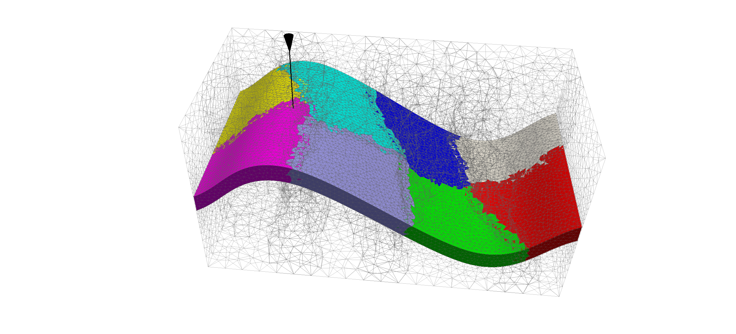
This mesh contains three continuous regions:
- a top region (overburden, elementary tag = 1).
- a middle region (reservoir layer, elementary tag = 2),
- a bottom region (underburden, elementary tag = 3).
A single injection wellbore is at the center of the reservoir. The picture shows an example of the 8-core METIS partitioning used to launch the simulation.
GEOSX input file
The XML file considered here follows the typical structure of the GEOSX input files:
Defining a solver
Let us inspect the Solver XML tags. It consists of 3 blocks CompositionalMultiphaseFlow, CompositionalMultiphaseWell and CompositionalMultiphaseReservoir, which are respectively handling the solution from multiphase flow in the reservoir, multiphase flow in the wells, and coupling between those two parts.
  <Solvers>
    <CompositionalMultiphaseReservoir
      name="coupledFlowAndWells"
      flowSolverName="compositionalMultiphaseFlow"
      wellSolverName="compositionalMultiphaseWell"
      logLevel="1"
      initialDt="1e2"
      targetRegions="{ Reservoir, wellRegion }">
      <NonlinearSolverParameters
        newtonTol="1.0e-3"
        lineSearchAction="None"
        maxTimeStepCuts="10"
        newtonMaxIter="40"/>
      <LinearSolverParameters
        solverType="direct"/>
    </CompositionalMultiphaseReservoir>

    <CompositionalMultiphaseFlow
      name="compositionalMultiphaseFlow"
      targetRegions="{ Reservoir }"
      discretization="fluidTPFA"
      fluidNames="{ fluid }"
      solidNames="{ rock }"
      relPermNames="{ relperm }"
      temperature="368.15"
      maxCompFractionChange="0.2"
      logLevel="1"
      useMass="1"/>

    <CompositionalMultiphaseWell
      name="compositionalMultiphaseWell"
      targetRegions="{ wellRegion }"
      fluidNames="{ fluid }"
      relPermNames="{ relperm }"
      wellTemperature="368.15"
      logLevel="1"
      useMass="1">
      <WellControls
        name="wellControls"
        type="injector"
        control="liquidRate"
        targetBHP="1e8"
        targetRate="50"
        injectionStream="{ 0.995, 0.005 }"/>
    </CompositionalMultiphaseWell>
  </Solvers>
In the CompositionalMultiphaseFlow (Compositional Multiphase Flow Solver), a classical multiphase compositional solver is detailed, including a TPFA discretization, reference to fluid data through fluidNames, to solid data through solidNames and to relative permeability models through relPermNames attributes.
The CompositionalMultiphaseWell (Compositional Multiphase Well Solver) consists of wellbore specifications (see Tutorial 4: Multiphase flow with wells for detailed tutorial on wells integration). As its reservoir counterpart, it includes references to fluid and relative permeability models, but also defines a WellControls sub-tag, that can specified injector and producer control splitting between BHP-controlled or rate-controlled. Alongside with that attribute are the targetBHP and targetRate that specify the maximal admissible pressure and rate for the well. The injector-specific attribute, injectionStream, describes the composition of the injected mixture.
The coupling section CompositionalMultiphaseReservoir describes the binding between those two previous elements (see Tutorial 8: Terzaghi’s poroelastic problem for detailed tutorial on coupling physics in GEOSX). In addition to being bound to the previously described blocks through flowSolverName and wellSolverName sub-tags, it contains the initialDt starting time-step size value and defines the NonlinearSolverParameters and LinearSolverParameters that are used to control Newton-loop and linear solver behaviors (see Linear Solvers for a detailed description of linear solvers attributes).
Specifying a computational mesh
The Mesh tag is used as in previous tutorials to import the field mesh either internally (Tutorial 1: First steps) or externally (Tutorial 2: Using an external mesh). In the current tutorial, this tag is also of paramount importance as it is where the InternalWell multi-segmented wells are defined. Apart from the name identifier attribute and their wellRegionName (ElementRegions) and wellControlsName (Solver) binding attributes, polylineNodeCoords and polylineSegmentConn attributes are used to define the path of the wellbore and connections between its nodes. The numElementsPerSegment is discretizing the wellbore segments while the radius attribute specifies the wellbore radius (Tutorial 4: Multiphase flow with wells for details on wellbore use). Once the wellbore is defined and discretized, the position of Perforations is defined using curvilinear distance from the head of the wellbore (distanceFromHead).
  <Mesh>
    <PAMELAMeshGenerator
      name="SyntheticMesh"
      file="synthetic.msh"/>

    <InternalWell
      name="wellInjector1"
      wellRegionName="wellRegion"
      wellControlsName="wellControls"
      meshName="SyntheticMesh"
      polylineNodeCoords="{ { 4500.0, 5000.0, 7500.0 },
                            { 4500.0, 5000.0, 7450.0 } }"
      polylineSegmentConn="{ { 0, 1 } }"
      radius="0.1"
      numElementsPerSegment="2">
      <Perforation
        name="injector1_perf1"
        distanceFromHead="45"/>
    </InternalWell>
  </Mesh>
Note
It is the responsibility of the user to make sure that there is a perforation in the bottom cell of the well mesh, otherwise an error will be thrown and the simulation will terminate.
Geometry tag
The Geometry XML block was used in single-phase tutorials to specify boundary conditions. Since we use wells and assume no-flow boundary conditions in this tutorial, the Geometry block is not needed.
Specifying events
The solver is applied as a periodic event whose target is referred to as Solvers/coupledFlowAndWells name-tag.
Using the maxEventDt attribute, we specify a max time step size of 1.5 x 10^6 seconds.
The output event triggers a vtk output every 10^7 seconds, constraining the solver schedule to match exactly these dates.
The output path to data is specified as a target of this PeriodicEvent.
An other periodic event is defined under the name restarts.
It consists of saved checkpoints every 5 x 10^6 seconds, whose physical output folder name is defined under the Output tag.
Finally, the time history collection and output events are used to trigger the mechanisms involved in the generation of a time series of well pressure (see the procedure outlined in Tasks Manager).
  <Events
    maxTime="5e5"> <!-- We will simulate more time (2.5e8 s) when the MGR solver is available by default -->

    <PeriodicEvent
      name="outputs"
      timeFrequency="1e7"
      targetExactTimestep="1"
      target="/Outputs/syntheticReservoirVizFile"/>

    <PeriodicEvent
      name="restarts"
      timeFrequency="5e7"
      targetExactTimestep="1"
      target="/Outputs/restartOutput"/>

    <PeriodicEvent
      name="timeHistoryCollection"
      timeFrequency="5e6"
      targetExactTimestep="1"
      target="/Tasks/wellPressureCollection" />

    <PeriodicEvent
      name="timeHistoryOutput"
      timeFrequency="2.5e8"
      targetExactTimestep="1"
      target="/Outputs/timeHistoryOutput" />

    <PeriodicEvent
      name="solverApplications"
      maxEventDt="1.5e6"
      target="/Solvers/coupledFlowAndWells"/>

  </Events>
Defining Numerical Methods
The TwoPointFluxApproximation is chosen as our fluid equation discretization. The tag specifies:
- A primary field to solve for as
fieldName. For a flow problem, this field is pressure. - A
fieldNameused to specify boundary objects with boundary conditions. - A
coefficientNameused for TPFA transmissibilities constructions.
Here, we specify targetRegions (we only solve flow equations in the reservoir portion of our model).
  <NumericalMethods>
    <FiniteVolume>
      <TwoPointFluxApproximation
        name="fluidTPFA"
        targetRegions="{ Reservoir }"
        fieldName="pressure"
        coefficientName="permeability"/>
    </FiniteVolume>
  </NumericalMethods>
Defining regions in the mesh
As in Tutorial 3: A simple field case, the ElementRegions tag allows us to distinguish the over- and underburden from the reservoir. The novelty here is the addition of WellElementRegions that are not bound to a cellBlock and contain a list of modeled materials.
  <ElementRegions>
    <CellElementRegion
      name="Reservoir"
      cellBlocks="{ Reservoir_TETRA }"
      materialList="{ fluid, rock, relperm }"/>

    <CellElementRegion
      name="Burden"
      cellBlocks="{ Overburden_TETRA, Underburden_TETRA }"
      materialList="{ rock }"/>

    <WellElementRegion
      name="wellRegion"
      materialList="{ fluid, relperm }"/>
  </ElementRegions>
Defining material properties with constitutive laws
Under the Constitutive tag, three items can be found:
- MultiPhaseMultiComponentFluid : this tag defines phase names, component molar weights and characteristic behaviors such as viscosity and density dependencies with respect to pressure and temperature.
- PoreVolumeCompressibleSolid : this tag contains all the data needed to model rock compressibility.
- BrooksCoreyRelativePermeability : this tag defines the relative permeability model for each phase, its end-point values, residual volume fractions (saturations), and Corey exponents.
  <Constitutive>
    <MultiPhaseMultiComponentFluid
      name="fluid"
      phaseNames="{ gas, water }"
      componentNames="{ co2, water }"
      componentMolarWeight="{ 44e-3, 18e-3 }"
      phasePVTParaFiles="{ pvt_tables/pvtgas.txt, pvt_tables/pvtliquid.txt }"
      flashModelParaFile="pvt_tables/co2flash.txt"/>

    <PoreVolumeCompressibleSolid
      name="rock"
      referencePressure="1e7"
      compressibility="4.5e-10"/>

    <BrooksCoreyRelativePermeability
      name="relperm"
      phaseNames="{ gas, water }"
      phaseMinVolumeFraction="{ 0.05, 0.30 }"
      phaseRelPermExponent="{ 2.0, 2.0 }"
      phaseRelPermMaxValue="{ 1.0, 1.0 }"/>
  </Constitutive>
One can notice that the PVT data specified by MultiPhaseMultiComponentFluid is set to model the behavior of CO2 in the liquid and gas phases as a function of pressure and temperature. These pvtgas.txt and pvtliquid.txt files are composed as follows:
DensityFun SpanWagnerCO2Density 1e6 1.5e7 5e4 94 96 1
ViscosityFun FenghourCO2Viscosity 1e6 1.5e7 5e4 94 96
DensityFun BrineCO2Density 1e6 1.5e7 5e4 94 96 1 0
ViscosityFun BrineViscosity 0
The first keyword is an identifier for either a density or a viscosity model, generated by GEOSX at runtime. It is followed by an identifier for the type of model (see Fluid Models). Then, the lower, upper and step increment values for pressure and temperature range are specified. The trailing 0 for BrineCO2Density entry is the salinity of the brine (see CO2 and brine models).
Note
The 0 value for BrineViscosity indicates that liquid CO2 viscosity is constant with respect to pressure and temperature.
Defining properties with the FieldSpecifications
As in previous tutorials, the FieldSpecifications tag is used to declare fields such as directional permeability, reference porosity, initial pressure, and compositions. Here, these fields are homogeneous, except for the permeability field that is taken from the 5th layer of the SPE10 test case and specified in Functions as in Tutorial 3: A simple field case.
  <FieldSpecifications>
    <FieldSpecification
      name="permx"
      initialCondition="1"
      component="0"
      setNames="{ all }"
      objectPath="ElementRegions/Reservoir"
      fieldName="permeability"
      scale="1e-14"
      functionName="permxFunc"/>

    <FieldSpecification
      name="permy"
      initialCondition="1"
      component="1"
      setNames="{ all }"
      objectPath="ElementRegions/Reservoir"
      fieldName="permeability"
      scale="1e-14"
      functionName="permyFunc"/>

    <FieldSpecification
      name="permz"
      initialCondition="1"
      component="2"
      setNames="{ all }"
      objectPath="ElementRegions/Reservoir"
      fieldName="permeability"
      scale="1e-17"
      functionName="permzFunc"/>

    <FieldSpecification
      name="referencePorosity"
      initialCondition="1"
      setNames="{ all }"
      objectPath="ElementRegions/Reservoir"
      fieldName="referencePorosity"
      scale="0.1"/>

    <FieldSpecification
      name="initialPressure"
      initialCondition="1"
      setNames="{ all }"
      objectPath="ElementRegions/Reservoir"
      fieldName="pressure"
      scale="4e7"/>

    <FieldSpecification
      name="initialComposition_co2"
      initialCondition="1"
      setNames="{ all }"
      objectPath="ElementRegions/Reservoir"
      fieldName="globalCompFraction"
      component="0"
      scale="0.0001"/>

    <FieldSpecification
      name="initialComposition_water"
      initialCondition="1"
      setNames="{ all }"
      objectPath="ElementRegions/Reservoir"
      fieldName="globalCompFraction"
      component="1"
      scale="0.9999"/>
  </FieldSpecifications>
Specifying output formats
The Outputs XML tag is used to write visualization, restart, and time history files.
Here, we write visualization files in a format natively readable by Paraview under the tag VTK. A Restart tag is also be specified. In conjunction with a PeriodicEvent, a restart file allows to resume computations from a set checkpoint in time. Finally, we require an output of the well pressure history using the TimeHistory tag.
  <Outputs>
    <VTK
      name="syntheticReservoirVizFile"/>

    <Restart
      name="restartOutput"/>

    <TimeHistory
      name="timeHistoryOutput"
      sources="{/Tasks/wellPressureCollection}"
      filename="wellPressureHistory" />

  </Outputs>
Specifying tasks
In the Events block, we have defined an event requesting that a task periodically collects the pressure at the well.
This task is defined here, in the PackCollection XML sub-block of the Tasks block.
The task contains the path to the object on which the field to collect is registered (here, a WellElementSubRegion) and the name of the field (here, pressure).
The details of the history collection mechanism can be found in Tasks Manager.
  <Tasks>
    <PackCollection
      name="wellPressureCollection"
      objectPath="ElementRegions/wellRegion/wellRegionuniqueSubRegion"
      fieldName="pressure" />

  </Tasks>
Running GEOSX
The simulation can be launched with on 8 cores using MPI-parallelism:
mpirun -np 8 geosx -i FieldCaseCo2InjTutorial.xml
Then, the multicore loading will rank-prefix the usual GEOSX mesh pre-treatment output as
1 >>> **********************************************************************
1 >>>                          PAMELA Library Import tool
1 >>> **********************************************************************
1 >>> GMSH FORMAT IDENTIFIED
1 >>> *** Importing Gmsh mesh format...
3 >>> **********************************************************************
6 >>> **********************************************************************
6 >>>                          PAMELA Library Import tool
6 >>> **********************************************************************
6 >>> GMSH FORMAT IDENTIFIED
3 >>>                          PAMELA Library Import tool
3 >>> **********************************************************************
3 >>> GMSH FORMAT IDENTIFIED
6 >>> *** Importing Gmsh mesh format...
3 >>> *** Importing Gmsh mesh format...
7 >>> **********************************************************************
7 >>>                          PAMELA Library Import tool
7 >>> **********************************************************************
7 >>> GMSH FORMAT IDENTIFIED
7 >>> *** Importing Gmsh mesh format...
0 >>> **********************************************************************
0 >>>                          PAMELA Library Import tool
0 >>> **********************************************************************
0 >>> GMSH FORMAT IDENTIFIED
0 >>> *** Importing Gmsh mesh format...
5 >>> **********************************************************************
5 >>>                          PAMELA Library Import tool
5 >>> **********************************************************************
5 >>> GMSH FORMAT IDENTIFIED
5 >>> *** Importing Gmsh mesh format...
4 >>> **********************************************************************
4 >>>                          PAMELA Library Import tool
4 >>> **********************************************************************
4 >>> GMSH FORMAT IDENTIFIED
4 >>> *** Importing Gmsh mesh format...
2 >>> **********************************************************************
2 >>>                          PAMELA Library Import tool
2 >>> **********************************************************************
2 >>> GMSH FORMAT IDENTIFIED
2 >>> *** Importing Gmsh mesh format...
7 >>> Reading nodes...
4 >>> Reading nodes...
1 >>> Reading nodes...
5 >>> Reading nodes...
0 >>> Reading nodes...
6 >>> Reading nodes...
3 >>> Reading nodes...
2 >>> Reading nodes...
6 >>> Done0
6 >>> Reading elements...
5 >>> Done0
5 >>> Reading elements...
4 >>> Done0
4 >>> Reading elements...
3 >>> Done0
3 >>> Reading elements...
1 >>> Done0
1 >>> Reading elements...
7 >>> Done0
7 >>> Reading elements...
0 >>> Done0
0 >>> Reading elements...
2 >>> Done0
A restart from a checkpoint file FieldCaseCo2InjTutorial_restart_000000015.root is always available thanks to the following command line :
mpirun -np 8 geosx -i FieldCaseCo2InjTutorial.xml -r FieldCaseCo2InjTutorial_restart_000000015
The output then shows the loading of HDF5 restart files by each core.
Loading restart file /work/simu/geosx/test/FieldCaseCo2InjTutorial_restart_000000015
Rank 0: rankFilePattern = /work/simu/geosx/test/FieldCaseCo2InjTutorial_restart_000000015/rank_%07d.hdf5
Rank 0: Reading in restart file at /work/simu/geosx/test/FieldCaseCo2InjTutorial_restart_000000015/rank_0000000.hdf5
Rank 4: Reading in restart file at /work/simu/geosx/test/FieldCaseCo2InjTutorial_restart_000000015/rank_0000004.hdf5
Rank 5: Reading in restart file at /work/simu/geosx/test/FieldCaseCo2InjTutorial_restart_000000015/rank_0000005.hdf5
Rank 7: Reading in restart file at /work/simu/geosx/test/FieldCaseCo2InjTutorial_restart_000000015/rank_0000007.hdf5
Rank 1: Reading in restart file at /work/simu/geosx/test/FieldCaseCo2InjTutorial_restart_000000015/rank_0000001.hdf5
Rank 3: Reading in restart file at /work/simu/geosx/test/FieldCaseCo2InjTutorial_restart_000000015/rank_0000003.hdf5
Rank 2: Reading in restart file at /work/simu/geosx/test/FieldCaseCo2InjTutorial_restart_000000015/rank_0000002.hdf5
Rank 6: Reading in restart file at /work/simu/geosx/test/FieldCaseCo2InjTutorial_restart_000000015/rank_0000006.hdf5
Visualization of results
Post-treating under Paraview, we can isolate the Reservoir block and focus on planes orthogonal to the injection wellbore.
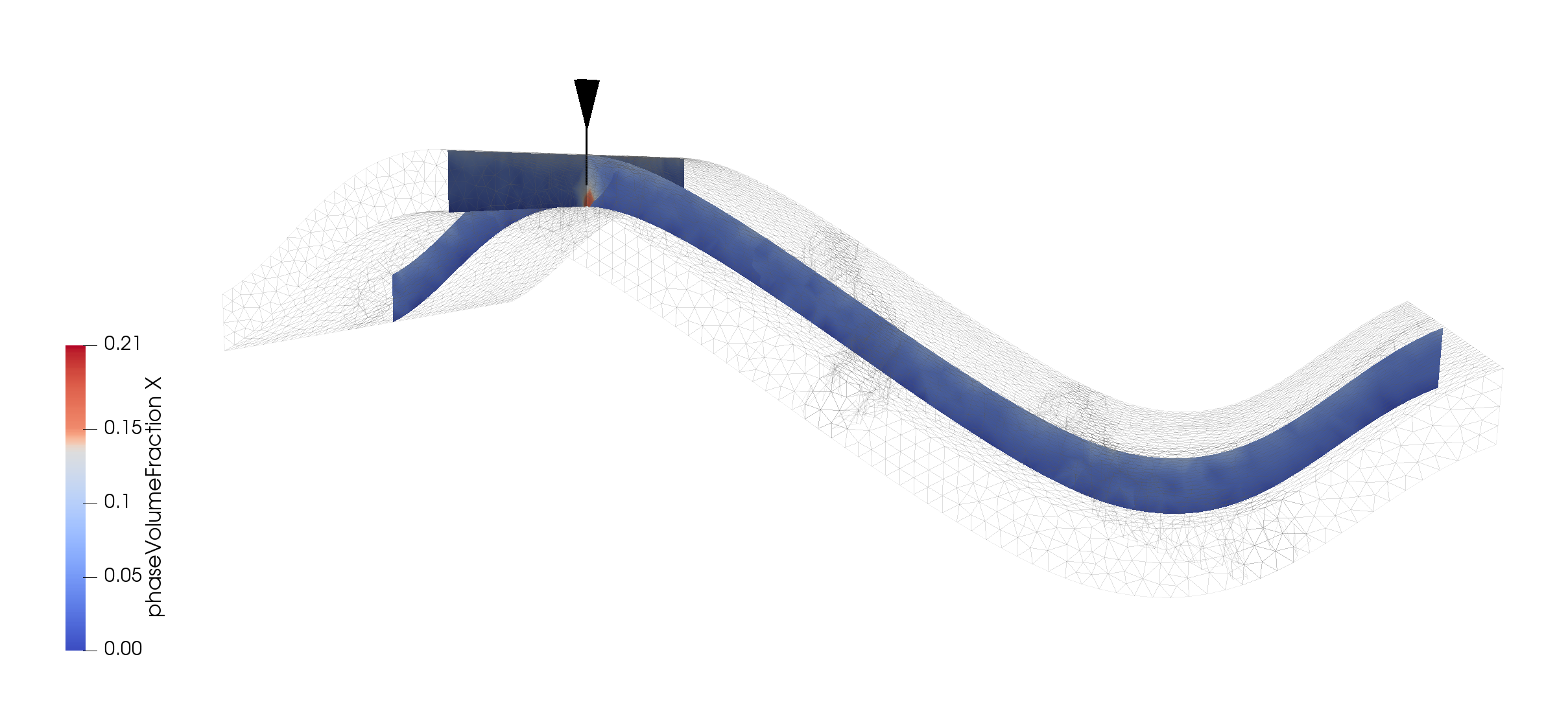
Closing up to the wellbore, we can see the reservoir filling up with CO 2,
Inspecting the pressure value along the same plane slices, we can check pressure rise at the injector
To go further
Feedback on this tutorial
This concludes the CO 2 injection field case tutorial. For any feedback on this tutorial, please submit a GitHub issue on the project’s GitHub page.
Next tutorial
In the next tutorial Tutorial 7: An elastic beam, we switch to mechanics and learn how to run a bending case to get familiar with mechanical problems in GEOSX.
For more details
- A complete description of the reservoir flow solver is found here: Compositional Multiphase Flow Solver.
- The well solver is described at Compositional Multiphase Well Solver.
- The available fluid constitutive models are listed at Fluid Models.