Tutorial 4: Multiphase flow with wells
Context
In this tutorial, we set up a multiphase, multicomponent test case (see Compositional Multiphase Flow Solver). The permeability field corresponds to the three bottom layers (layers 83, 84, and 85) of the SPE10 test case. The thermodynamic behavior of the fluid mixture is specified using a Dead-Oil model. Injection and production are performed using multi-segmented wells.
Objectives
At the end of this tutorial you will know:
- how to import an external mesh with embedded geological properties (porosity and permeability) in the Eclipse format (
.grdecl),- how to set up a multiphase, multicomponent simulation,
- how to couple reservoir flow with wells.
Input file
This tutorial is based on the XML file located at
src/coreComponents/physicsSolvers/fluidFlow/benchmarks/SPE10/dead_oil_spe10_layers_83_84_85.xml
The mesh file used in this tutorial is not stored in the main GEOSX repository. To run the test case specified in the XML file, you must first download the GEOSXDATA repository. The XML file that we are going to describe assumes that the GEOSXDATA repository has been cloned in the same folder as the GEOSX repository.
Note
GEOSXDATA is a separate repository in which we store large mesh files in order to keep the main GEOSX repository lightweight.
GEOSX input file
The XML file considered here follows the typical structure of the GEOSX input files:
Solvers: coupling reservoir flow with wells
In GEOSX, the simulation of reservoir flow with wells is set up by combining three solvers listed and parameterized in the Solvers XML block of the input file. We introduce separately a flow solver and a well solver acting on different regions of the domain—respectively, the reservoir region and the well regions. To drive the simulation and bind these single-physics solvers, we also specify a coupling solver between the reservoir flow solver and the well solver. This coupling of single-physics solvers is the generic approach used in GEOSX to define multiphysics problems. It is illustrated in Tutorial 8: Terzaghi’s poroelastic problem for a poroelastic test case.
The three solvers employed in this tutorial are:
- the single-physics reservoir flow solver, a solver of type CompositionalMultiphaseFlow named
compositionalMultiphaseFlow(more information on this solver at Compositional Multiphase Flow Solver),- the single-physics well solver, a solver of type CompositionalMultiphaseWell named
compositionalMultiphaseWell(more information on this solver at Compositional Multiphase Well Solver),- the coupling solver that binds the two single-physics solvers above, an object of type CompositionalMultiphaseReservoir named
coupledFlowAndWells.
Let us have a closer look at the Solvers XML block displayed below.
Each solver has a name that can be chosen by the user and is not imposed by GEOSX.
These names are used here to point the coupling solver to the single-physics solvers
using the attributes flowSolverName and wellSolverName. The name of the coupling
solver is also used in the Events XML block to trigger the application of the solver.
The coupling solver defines all the target regions on which the single-physics solvers
are applied, namely the reservoir region (named reservoir here) and one region for each well.
The simulation is fully coupled and driven by the coupled solver. Therefore, the time stepping
information (here, initialDt, but there may be other parameters used to fine-tune the time
stepping strategy), the nonlinear solver parameters, and the linear solver parameters must be
specified at the level of the coupling solver. There is no need to specify these parameters at
the level of the single-physics solvers.
Note that it is worth repeating the logLevel=1 parameter at the level of the well solver
to make sure that a notification is issued when the well control is switched (from rate control
to BHP control, for instance).
Note that the same fluid and relative permeability
models (set with the fluidNames and relPermNames attributes) must be used in the two
single-physics solvers.
GEOSX will throw an error and terminate the simulation if it is not the case.
Take note of the specification of well constraints and controls in the single-physics
well solver with control, targetBHP, targetRate
and injectionStream (for the composition of the multiphase injection fluid).
  <Solvers>
    <CompositionalMultiphaseReservoir
      name="coupledFlowAndWells"
      flowSolverName="compositionalMultiphaseFlow"
      wellSolverName="compositionalMultiphaseWell"
      logLevel="1"
      initialDt="1e3"
      targetRegions="{ reservoir, wellRegion1, wellRegion2, wellRegion3, wellRegion4, wellRegion5 }">
      <NonlinearSolverParameters
        newtonTol="1.0e-4"
        dtIncIterLimit="0.4"
        maxTimeStepCuts="10"
        lineSearchAction="None"
        newtonMaxIter="20"/>
      <!-- Note that the direct solver is quite slow -->
      <!-- This block will be updated when Hypre becomes the default  -->
      <LinearSolverParameters
        solverType="direct"/>
    </CompositionalMultiphaseReservoir>

    <CompositionalMultiphaseFlow
      name="compositionalMultiphaseFlow"
      targetRegions="{ reservoir }"
      discretization="fluidTPFA"
      fluidNames="{ fluid }"
      solidNames="{ rock }"
      relPermNames="{ relperm }"
      maxCompFractionChange="0.3"
      temperature="297.15"
      useMass="1"/>

    <CompositionalMultiphaseWell
      name="compositionalMultiphaseWell"
      targetRegions="{ wellRegion1, wellRegion2, wellRegion3, wellRegion4, wellRegion5 }"
      fluidNames="{ fluid }"
      relPermNames="{ relperm }"
      wellTemperature="297.15"
      maxCompFractionChange="0.3"
      logLevel="1"
      useMass="1">
      <WellControls
        name="wellControls1"
        type="producer"
        control="BHP"
        targetBHP="2.7579e7"
        targetRate="1e9"/>
      <WellControls
        name="wellControls2"
        type="producer"
        control="BHP"
        targetBHP="2.7579e7"
        targetRate="1e9"/>
      <WellControls
        name="wellControls3"
        type="producer"
        control="BHP"
        targetBHP="2.7579e7"
        targetRate="1e9"/>
      <WellControls
        name="wellControls4"
        type="producer"
        control="BHP"
        targetBHP="2.7579e7"
        targetRate="1e9"/>
      <WellControls
        name="wellControls5"
        type="injector"
        control="liquidRate"
        targetBHP="6.8948e9"
        targetRate="1e0"
        injectionStream="{ 0.0, 0.0, 1.0 }"/>
    </CompositionalMultiphaseWell>
  </Solvers>
Specifying a reservoir mesh and defining the geometry of the wells
In the presence of wells, the Mesh block of the XML input file includes two parts:
- a sub-block PAMELAMeshGenerator defining the reservoir mesh (see Tutorial 2: Using an external mesh for more on this),
- a collection of sub-blocks InternalWell defining the geometry of the wells.
In this tutorial, the reservoir mesh is imported from an Eclipse .grdecl mesh file that
describes the mesh. It also contains the value of the three components of the permeability
(in the x, y, and z directions) and the value of the porosity for each cell.
The import is requested in the PAMELAMeshGenerator XML sub-block. The mesh description
must be done in meters, and the permeability field must be specified in square meters (not in Darcy or milliDarcy).
More information about the mesh importer can be found in Meshes.
Each well is defined internally (i.e., not imported from a file) in a separate InternalWell
XML sub-block. An InternalWell sub-block must point to the reservoir mesh that the well perforates
using the attribute meshName, to the region corresponding to this well using the attribute
wellRegionName, and to the control of this well using the attribute wellControl.
In this tutorial, the five wells have the same structure, with one vertical segment
discretized into four well cells.
We define three perforations along the well (one perforation for each layer of the reservoir mesh).
The location of the perforations is found internally using the linear distance along the wellbore
from the top of the well, specified by the attribute distanceFromHead.
It is the responsibility of the user to make sure that there is a perforation in the bottom cell
of the well mesh otherwise an error will be thrown and the simulation will terminate. The well
geometry must be specified in meters.
  <Mesh>
    <PAMELAMeshGenerator
      name="mesh"
      file="../../../../../../../GEOSXDATA/DataSets/SPE10/EclipseBottomLayers/SPE10_LAYERS_83_84_85.GRDECL"
      fieldsToImport="{ PERM, PORO }"
      fieldNamesInGEOSX="{ permeability, referencePorosity }"/>

    <InternalWell
      name="wellProducer1"
      wellRegionName="wellRegion1"
      wellControlsName="wellControls1"
      meshName="mesh"
      polylineNodeCoords="{ { 0.1, 0.1, 3710.03 },
                            { 0.1, 0.1, 3707.59 } }"
      polylineSegmentConn="{ { 0, 1 } }"
      radius="0.1"
      numElementsPerSegment="4">
      <Perforation
        name="producer1_perf1"
        distanceFromHead="0.91"/>
      <Perforation
        name="producer1_perf2"
        distanceFromHead="1.52"/>
      <Perforation
        name="producer1_perf3"
        distanceFromHead="2.13"/>
    </InternalWell>

    <InternalWell
      name="wellProducer2"
      wellRegionName="wellRegion2"
      wellControlsName="wellControls2"
      meshName="mesh"
      polylineNodeCoords="{ { 365.7, 0.1, 3710.03 },
                            { 365.7, 0.1, 3707.59 } }"
      polylineSegmentConn="{ { 0, 1 } }"
      radius="0.1"
      numElementsPerSegment="4">
      <Perforation
        name="producer2_perf1"
        distanceFromHead="0.91"/>
      <Perforation
        name="producer2_perf2"
        distanceFromHead="1.52"/>
      <Perforation
        name="producer2_perf3"
        distanceFromHead="2.13"/>
    </InternalWell>

    <InternalWell
      name="wellProducer3"
      wellRegionName="wellRegion3"
      wellControlsName="wellControls3"
      meshName="mesh"
      polylineNodeCoords="{ { 365.7, 670.5, 3710.03 },
                            { 365.7, 670.5, 3707.59 } }"
      polylineSegmentConn="{ { 0, 1 } }"
      radius="0.1"
      numElementsPerSegment="4">
      <Perforation
        name="producer3_perf1"
        distanceFromHead="0.91"/>
      <Perforation
        name="producer3_perf2"
        distanceFromHead="1.52"/>
      <Perforation
        name="producer3_perf3"
        distanceFromHead="2.13"/>
    </InternalWell>

    <InternalWell
      name="wellProducer4"
      wellRegionName="wellRegion4"
      wellControlsName="wellControls4"
      meshName="mesh"
      polylineNodeCoords="{ { 0.1, 670.5, 3710.03 },
                            { 0.1, 670.5, 3707.59 } }"
      polylineSegmentConn="{ { 0, 1 } }"
      radius="0.1"
      numElementsPerSegment="4">
      <Perforation
        name="producer4_perf1"
        distanceFromHead="0.91"/>
      <Perforation
        name="producer4_perf2"
        distanceFromHead="1.52"/>
      <Perforation
        name="producer4_perf3"
        distanceFromHead="2.13"/>
    </InternalWell>

    <InternalWell
      name="wellInjector1"
      wellRegionName="wellRegion5"
      wellControlsName="wellControls5"
      meshName="mesh"
      polylineNodeCoords="{ { 182.8, 335.2, 3710.03 },
                            { 182.8, 335.2, 3707.59 } }"
      polylineSegmentConn="{ { 0, 1 } }"
      radius="0.1"
      numElementsPerSegment="4">
      <Perforation
        name="injector1_perf1"
        distanceFromHead="0.91"/>
      <Perforation
        name="injector1_perf2"
        distanceFromHead="1.52"/>
      <Perforation
        name="injector1_perf3"
        distanceFromHead="2.13"/>
    </InternalWell>
  </Mesh>
Geometry tag
The Geometry XML block was used in the previous tutorials to specify boundary conditions. Since we use wells and assume no-flow boundary conditions in this tutorial, the Geometry block is not needed.
Specifying events
In the Events XML block of this tutorial, we specify five types of PeriodicEvents serving different purposes: solver application, result output, restart file generation, time history collection and output.
The periodic event named solverApplications triggers the application of the solvers
on their target regions.
For a coupled simulation, this event must point to the coupling solver by name.
The name of the coupling solver is coupledFlowAndWells and was defined in the Solvers block.
The time step is initialized using the initialDt attribute of the coupling solver.
Then, if the solver converges in more than a certain number of nonlinear iterations (by default, 40% of the
maximum number of nonlinear iterations), the time step will be increased until it reaches the maximum
time step size specified with maxEventDt.
If the time step fails, the time step will be cut. The parameters defining the time stepping strategy
can be finely tuned by the user in the coupling solver block.
Note that all times are in seconds.
The output event forces GEOSX to write out the results at the frequency specified by the attribute
timeFrequency.
Here, we choose to output the results using the VTK format (see Tutorial 2: Using an external mesh
for a tutorial that uses the Silo output file format).
Using targetExactTimestep=1 in this XML block forces GEOSX to adapt the time stepping to
ensure that an output is generated exactly at the time frequency requested by the user.
In the target attribute, we must use the name defined in the VTK XML tag
inside the Output XML section, as documented at the end of this tutorial (here, vtkOutput).
The restart event instructs GEOSX to write out one or multiple restart files at set times in the simulation.
Restart files are used to restart a simulation from a specific point in time.
These files contain all the necessary information to restoring all internal
variables to their exact state at the chosen time, and continue the simulation from here on.
Here, the target attribute must contain the name defined in the Restart XML sub-block
of the Output XML block (here, restartOutput).
The time history collection events instruct GEOSX to collect the rates of each producing well at a given frequency.
Using the target attribute, each collection event must point by name to a specific task defined in the PackCollection XML sub-block of the Tasks XML block discussed later (here, timeHistoryCollection1 for the first well).
Finally, the time history output events instruct GEOSX when to output (i.e., write to an HDF5 file) the data collected by the task mentioned above. The target attribute points to the TimeHistory sub-block of the Outputs block (here, timeHistoryOutput1 for the first well).
More information about events can be found at Event Management.
  <Events
    maxTime="1.5e7">

    <PeriodicEvent
      name="vtk"
      timeFrequency="2e6"
      targetExactTimestep="1"
      target="/Outputs/vtkOutput"/>

    <PeriodicEvent
      name="restarts"
      timeFrequency="5529600"
      targetExactTimestep="1"
      target="/Outputs/restartOutput"/>

    <PeriodicEvent
      name="timeHistoryOutput1"
      timeFrequency="1.5e7"
      targetExactTimestep="1"
      target="/Outputs/timeHistoryOutput1" />

    <PeriodicEvent
      name="timeHistoryOutput2"
      timeFrequency="1.5e7"
      targetExactTimestep="1"
      target="/Outputs/timeHistoryOutput2" />

    <PeriodicEvent
      name="timeHistoryOutput3"
      timeFrequency="1.5e7"
      targetExactTimestep="1"
      target="/Outputs/timeHistoryOutput3" />

    <PeriodicEvent
      name="timeHistoryOutput4"
      timeFrequency="1.5e7"
      targetExactTimestep="1"
      target="/Outputs/timeHistoryOutput4" />

    <PeriodicEvent
      name="solverApplications"
      maxEventDt="2e5"
      target="/Solvers/coupledFlowAndWells"/>

    <PeriodicEvent
      name="timeHistoryCollection1"
      timeFrequency="5e5"
      targetExactTimestep="1"
      target="/Tasks/wellRateCollection1" />

    <PeriodicEvent
      name="timeHistoryCollection2"
      timeFrequency="5e5"
      targetExactTimestep="1"
      target="/Tasks/wellRateCollection2" />

    <PeriodicEvent
      name="timeHistoryCollection3"
      timeFrequency="5e5"
      targetExactTimestep="1"
      target="/Tasks/wellRateCollection3" />

    <PeriodicEvent
      name="timeHistoryCollection4"
      timeFrequency="5e5"
      targetExactTimestep="1"
      target="/Tasks/wellRateCollection4" />

  </Events>
Defining Numerical Methods
In the NumericalMethods XML block, we select a two-point flux approximation (TPFA) finite-volume scheme to discretize the governing equations on the reservoir mesh. TPFA is currently the only numerical scheme that can be used with a flow solver of type CompositionalMultiphaseFlow. There is no numerical scheme to specify for the well mesh.
  <NumericalMethods>
    <FiniteVolume>
      <TwoPointFluxApproximation
        name="fluidTPFA"
        fieldName="pressure"
        coefficientName="permeability"/>
    </FiniteVolume>
  </NumericalMethods>
Defining reservoir and well regions
In the presence of wells, it is required to specify at least two types of element regions in the ElementRegions XML block: CellElementRegion and WellElementRegion.
Here, we define a CellElementRegion named reservoir corresponding to the
reservoir mesh.
The attribute cellBlocks must be set to DEFAULT_HEX to point this element region
to the hexahedral mesh corresponding to the bottom layers of SPE10 that was
imported with the PAMELAMeshGenerator.
Note that DEFAULT_HEX is a name internally defined by the mesh importer to denote the only
hexahedral region of the reservoir mesh.
We refer to Tutorial 2: Using an external mesh for a discussion on
hexahedral meshes in GEOSX.
Note
If you use a name that is not DEFAULT_HEX for this attribute, GEOSX will throw an error at the beginning of the simulation.
The CellElementRegion must also point to the constitutive models that are used to update
the dynamic rock and fluid properties in the cells of the reservoir mesh.
The names fluid, rock, and relperm used for this in the materialList
correspond to the attribute name of the Constitutive block.
We also define five WellElementRegions corresponding to the five wells. These regions point to the well meshes defined in the Mesh XML block and to the constitutive models introduced in the Constitutive block. As before, this is done using the names chosen by the user when these blocks are defined.
  <ElementRegions>
    <CellElementRegion
      name="reservoir"
      cellBlocks="{ DEFAULT_HEX }"
      materialList="{ fluid, rock, relperm }"/>

    <WellElementRegion
      name="wellRegion1"
      materialList="{ fluid, relperm }"/>

    <WellElementRegion
      name="wellRegion2"
      materialList="{ fluid, relperm }"/>

    <WellElementRegion
      name="wellRegion3"
      materialList="{ fluid, relperm }"/>

    <WellElementRegion
      name="wellRegion4"
      materialList="{ fluid, relperm }"/>

    <WellElementRegion
      name="wellRegion5"
      materialList="{ fluid, relperm }"/>
  </ElementRegions>
Defining material properties with constitutive laws
For a simulation performed with the CompositionalMultiphaseFlow physics solver, at least three types of constitutive models must be specified in the Constitutive XML block:
- a fluid model describing the thermodynamics behavior of the fluid mixture,
- a relative permeability model,
- a rock compressibility model.
All these models use SI units exclusively. A capillary pressure model can also be specified in this block but is omitted here for simplicity.
Here, we introduce a fluid model describing a simplified mixture thermodynamic behavior.
Specifically, we use a Dead-Oil model by placing the XML tag BlackOilFluid with the attribute
fluidType=DeadOil. Other fluid models can be used with the CompositionalMultiphaseFlow
solver, as explained in Fluid Models.
With the tag BrooksCoreyRelativePermeability, we define a relative permeability model. A list of available relative permeability models can be found at Relative Permeability Models.
The properties are chosen to match those of the original SPE10 test case. Note that the current fluid model implemented in GEOSX only supports unit viscosities (i.e., 0.001 Pa.s). Therefore, we set the end point of the oil relative permeability to 0.1 to preserve the mobility ratio of the SPE10 test case.
Note
The names and order of the phases listed for the attribute phaseNames must be identical in the fluid model (here, BlackOilFluid) and the relative permeability model (here, BrooksCoreyRelativePermeability). Otherwise, GEOSX will throw an error and terminate.
We also introduce a model to define the rock compressibility. This step is similar to what is described in the previous tutorials (see for instance Tutorial 1: First steps).
We remind the reader that the attribute name of the constitutive models defined here
must be used in the ElementRegions and Solvers XML blocks to point the element
regions and the physics solvers to their respective constitutive models.
  <Constitutive>
    <BlackOilFluid
      name="fluid"
      fluidType="DeadOil"
      phaseNames="{ oil, gas, water }"
      surfaceDensities="{ 848.9, 0.9907, 1025.2 }"
      componentMolarWeight="{ 114e-3, 16e-3, 18e-3 }"
      tableFiles="{ pvdo.txt, pvdg.txt, pvtw.txt }"/>

    <BrooksCoreyRelativePermeability
      name="relperm"
      phaseNames="{ oil, gas, water }"
      phaseMinVolumeFraction="{ 0.2, 0.0, 0.2 }"
      phaseRelPermExponent="{ 2.0, 2.0, 2.0 }"
      phaseRelPermMaxValue="{ 0.1, 1.0, 1.0 }"/>

    <PoreVolumeCompressibleSolid
      name="rock"
      referencePressure="1e7"
      compressibility="1e-10"/>
  </Constitutive>
Defining properties with the FieldSpecifications
In the FieldSpecifications section, we define the initial conditions as well as the geological properties not read from the mesh file, such as the porosity field in this tutorial. All this is done using SI units. Here, we focus on the specification of the initial conditions for a simulation performed with the CompositionalMultiphaseFlow solver. We refer to Tutorial 1: First steps for a more general discussion on the FieldSpecification XML blocks.
For a simulation performed with the CompositionalMultiphaseFlow solver,
we have to set the initial pressure as well as the initial global component
fractions (in this case, the oil, gas, and water component fractions).
The component attribute of the FieldSpecification XML block must use the
order in which the phaseNames have been defined in the BlackOilFluid
XML block. In other words, component=0 is used to initialize the oil
global component fraction, component=1 is used to initialize the gas global
component fraction, and component=2 is used to initialize the water global
component fraction, because we previously set phaseNames="{oil, gas, water}"
in the BlackOilFluid XML block. Since the SPE10 test case only involves
two-phase flow, we set the initial component fraction of gas to zero.
There is no initialization to perform in the wells since the well properties are initialized internally using the reservoir initial conditions.
  <FieldSpecifications>
    <FieldSpecification
      name="initialPressure"
      initialCondition="1"
      setNames="{ all }"
      objectPath="ElementRegions/reservoir/DEFAULT_HEX"
      fieldName="pressure"
      scale="4.1369e7"/>

    <FieldSpecification
      name="initialComposition_oil"
      initialCondition="1"
      setNames="{ all }"
      objectPath="ElementRegions/reservoir/DEFAULT_HEX"
      fieldName="globalCompFraction"
      component="0"
      scale="1.0"/>

    <FieldSpecification
      name="initialComposition_gas"
      initialCondition="1"
      setNames="{ all }"
      objectPath="ElementRegions/reservoir/DEFAULT_HEX"
      fieldName="globalCompFraction"
      component="1"
      scale="0.0"/>

    <FieldSpecification
      name="initialComposition_water"
      initialCondition="1"
      setNames="{ all }"
      objectPath="ElementRegions/reservoir/DEFAULT_HEX"
      fieldName="globalCompFraction"
      component="2"
      scale="0.0"/>
  </FieldSpecifications>
Specifying the output formats
In this section, we request an output of the results in VTK format, an output of the restart file, and the output of the well rate history to four HDF5 files (one for each producer). Note that the names defined here must match the names used in the Events XML block to define the output frequency.
  <Outputs>
    <VTK
      name="vtkOutput"/>

    <Restart
      name="restartOutput"/>

    <TimeHistory
      name="timeHistoryOutput1"
      sources="{/Tasks/wellRateCollection1}"
      filename="wellRateHistory1" />

    <TimeHistory
      name="timeHistoryOutput2"
      sources="{/Tasks/wellRateCollection2}"
      filename="wellRateHistory2" />

    <TimeHistory
      name="timeHistoryOutput3"
      sources="{/Tasks/wellRateCollection3}"
      filename="wellRateHistory3" />

    <TimeHistory
      name="timeHistoryOutput4"
      sources="{/Tasks/wellRateCollection4}"
      filename="wellRateHistory4" />

  </Outputs>
Specifying tasks
In the Events block, we have defined four events requesting that a task periodically collects the rate for each producing well.
This task is defined here, in the PackCollection XML sub-block of the Tasks block.
The task contains the path to the object on which the field to collect is registered (here, a WellElementSubRegion) and the name of the field (here, wellElementMixtureConnectionRate).
The details of the history collection mechanism can be found in Tasks Manager.
  <Tasks>
    <PackCollection
      name="wellRateCollection1"
      objectPath="ElementRegions/wellRegion1/wellRegion1uniqueSubRegion"
      fieldName="wellElementMixtureConnectionRate" />
    <PackCollection
      name="wellRateCollection2"
      objectPath="ElementRegions/wellRegion2/wellRegion2uniqueSubRegion"
      fieldName="wellElementMixtureConnectionRate" />
    <PackCollection
      name="wellRateCollection3"
      objectPath="ElementRegions/wellRegion3/wellRegion3uniqueSubRegion"
      fieldName="wellElementMixtureConnectionRate" />
    <PackCollection
      name="wellRateCollection4"
      objectPath="ElementRegions/wellRegion4/wellRegion4uniqueSubRegion"
      fieldName="wellElementMixtureConnectionRate" />

  </Tasks>
All elements are now in place to run GEOSX.
Running GEOSX
The first few lines appearing to the console are indicating that the XML elements are read and registered correctly:
Adding Solver of type CompositionalMultiphaseReservoir, named coupledFlowAndWells
Adding Solver of type CompositionalMultiphaseFlow, named compositionalMultiphaseFlow
Adding Solver of type CompositionalMultiphaseWell, named compositionalMultiphaseWell
Adding Mesh: PAMELAMeshGenerator, mesh
Adding Mesh: InternalWell, wellProducer1
Adding Mesh: InternalWell, wellProducer2
Adding Mesh: InternalWell, wellProducer3
Adding Mesh: InternalWell, wellProducer4
Adding Mesh: InternalWell, wellInjector1
Adding Event: PeriodicEvent, solverApplications
Adding Event: PeriodicEvent, vtk
Adding Event: PeriodicEvent, restarts
Adding Output: VTK, vtkOutput
Adding Output: Restart, restartOutput
Adding Object CellElementRegion named reservoir from ObjectManager::Catalog.
Adding Object WellElementRegion named wellRegion1 from ObjectManager::Catalog.
Adding Object WellElementRegion named wellRegion2 from ObjectManager::Catalog.
Adding Object WellElementRegion named wellRegion3 from ObjectManager::Catalog.
Adding Object WellElementRegion named wellRegion4 from ObjectManager::Catalog.
Adding Object WellElementRegion named wellRegion5 from ObjectManager::Catalog.
This is followed by the creation of the 39600 hexahedral cells of the imported mesh:
0 >>> **********************************************************************
0 >>>                          PAMELA Library Import tool
0 >>> **********************************************************************
0 >>> ECLIPSE GRDECL FORMAT IDENTIFIED
0 >>> *** Importing Eclipse mesh format file bottom_layers_of_SPE10
0 >>> ---- Parsing bottom_layers_of_SPE10.grdecl
0 >>>      o SPECGRID or DIMENS Found
0 >>>      o COORD Found
0 >>>      o ZCORN Found
0 >>>      o PORO Found
0 >>>      o PERMX Found
0 >>>      o PERMY Found
0 >>>      o PERMZ Found
0 >>> *** Converting into internal mesh format
0 >>> 39600  total GRDECL hexas
0 >>> 39600  initially set as active hexas
0 >>> 0  active but flat hexas (->deactivated)
0 >>> 0  active but ill-shaped hexas (->deactivated)
0 >>> 0  duplicated hexas
0 >>> 39600  will actually be used in the GEOSX mesh
0 >>> *** Filling mesh with imported properties
0 >>> *** Creating Polygons from Polyhedra...
0 >>> 132840 polygons have been created
0 >>> *** Done
0 >>> *** Perform partitioning...
0 >>> TRIVIAL partitioning...
0 >>> Ghost elements...
0 >>> Clean mesh...
0 >>> *** Done...
0 >>> Clean Adjacency...
0 >>> *** Done...
When Running simulation is shown, we are done with the case set-up and
the code steps into the execution of the simulation itself:
Time: 0s, dt:1000s, Cycle: 0
  Attempt:  0, NewtonIter:  0
  ( R ) = ( 6.88e+04 ) ;
  Attempt:  0, NewtonIter:  1
  ( R ) = ( 2.73e+03 ) ;
  Last LinSolve(iter,res) = (   1, 2.22e-16 ) ;
  Attempt:  0, NewtonIter:  2
  ( R ) = ( 3.60e+00 ) ;
  Last LinSolve(iter,res) = (   1, 2.22e-16 ) ;
  Attempt:  0, NewtonIter:  3
  ( R ) = ( 1.30e-02 ) ;
  Last LinSolve(iter,res) = (   1, 2.22e-16 ) ;
  Attempt:  0, NewtonIter:  4
  ( R ) = ( 3.65e-07 ) ;
  Last LinSolve(iter,res) = (   1, 2.22e-16 ) ;
coupledFlowAndWells: Newton solver converged in less than 8 iterations, time-step required will be doubled.
Visualization of results
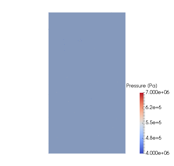
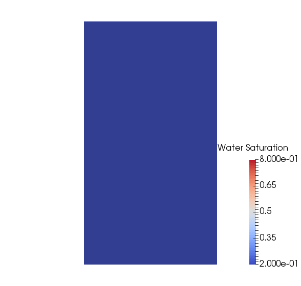
A file compatible with Paraview is produced in this tutorial. It is found in the output folder, and usually has the extension .pvd. More details about this file format can be found here. We can load this file into Paraview directly and visualize results:
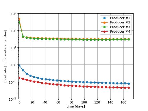
Using the time series output by GEOSX, we can extract the well rates. The script and image below illustrate how to post-process the hdf5 file to extract and plot useful information. Note that the difference in rates shown below can be explained by the fact that two producers are located in high-permeability regions, while the two other producers are located in very low permeability regions.
To go further
Feedback on this tutorial
This concludes the tutorial on setting up a Dead-Oil simulation in a channelized permeability field. For any feedback on this tutorial, please submit a GitHub issue on the project’s GitHub page.
Next tutorial
In Tutorial 5: Multiphase flow in the Egg model, we learn how to run a test case based on the Egg model.
For more details
- A complete description of the reservoir flow solver is found here: Compositional Multiphase Flow Solver.
- The well solver is description at Compositional Multiphase Well Solver.
- The available constitutive models are listed at Constitutive Models.