Tutorial 2: Using an external mesh¶

Context

In this tutorial, we use a simple single-phase flow solver (see Singlephase Flow Solver) to solve for pressure propagation on a mesh that is imported into GEOSX. The main goal of this tutorial is to learn how to work with external meshes, and to learn how easy it is to swap meshes on the same physical problem in GEOSX. This makes GEOSX a powerful tool to solve real field applications with complex geometries and perform assessments of mesh geometry and resolution effects.

Objectives

At the end of this tutorial you will know:

the syntax and format of input meshes,

how to input external files into a GEOSX input XML file,

how to run the same physical problem with two different meshes,

how to use and visualize hexahedral and tetrahedral meshes.

Input Files

This tutorial uses an XML file containing the main input for GEOSX and a separate file with all the mesh information. As we will see later, the main XML file points to the external mesh file with an include statement. The XML input file for this test case is located at:

src/coreComponents/physicsSolvers/fluidFlow/integratedTests/singlePhaseFlow/pamela_test/3D_10x10x10_compressible_pamela_hex_gravity.xml

The mesh file format used in this tutorial is called MSH. This format is a standard scientific meshing format not specific to GEOSX. It is maintained as the native format of the meshing tool Gmsh. MSH is designed for unstructured meshes and contains a compact and complete representation of the mesh geometry and of its properties. The mesh file used here is human-readable ASCII. It contains a list of nodes with their (x,y,z) coordinates, and a list of elements that are constructed from these nodes.

Hexahedral elements¶

In the first part of the tutorial, we will run flow simulations on a mesh made of hexahedral elements. These types of elements are used in classical cartesian grids (sugar cubes) or corner-point grids or pillar grids.

Brief discussion about hexahedral meshes in GEOSX¶

Although closely related, the hexahedral grids that GEOSX can process are slightly different than either structured grid or corner-point grids. The differences are worth pointing out here. In GEOSX:

hexahedra can have irregular shapes: no pillars are needed and vertices can be anywhere in space. This is useful for grids that turn, fold, or are heavily bent. Hexahedral blocks should nevertheless not be deprecated and have 8 distinct vertices. Some tolerance exists for deprecation to wedges or prisms in some solvers (finite element solvers), but it is best to avoid such situations and label elements according to their actual shape. Butterfly cells, flat cells, negative or zero volume cells will cause problems.

the mesh needs to be conformal: in 3D, this means that neighboring grid blocks have to share exactly a complete face. Note that corner-point grids do not have this requirement and neighboring blocks can be offset. When importing grids from commonly-used geomodeling packages, this is an important consideration. This problem is solved by splitting shifted grid blocks to restore conformity. While it may seem convenient to be able to have offset grid blocks at first, the advantages of conformal grids used in GEOSX are worth the extra meshing effort: by using conformal grids, GEOSX can run finite element and finite volume simulations on the same mesh without problems, going seamlessly from one numerical method to the other. This is key to enabling multiphysics simulation.

there is no assumption of overall structure: GEOSX does not need to know a number of block in the X, Y, Z direction (no NX, NY, NZ) and does not assume that the mesh is a full cartesian domain that the interesting parts of the reservoir must be carved out from. Blocks are numbered by indices that assume nothing about spatial positioning and there is no concept of (i,j,k). This approach also implies that no “masks” are needed to remove inactive or dead cells, as often done in cartesian grids to get the actual reservoir contours from a bounding box, and here we only need to specify grid blocks that are active. For performance and flexibility, this lean approach to meshes is important.

Importing an external mesh with PAMELA¶

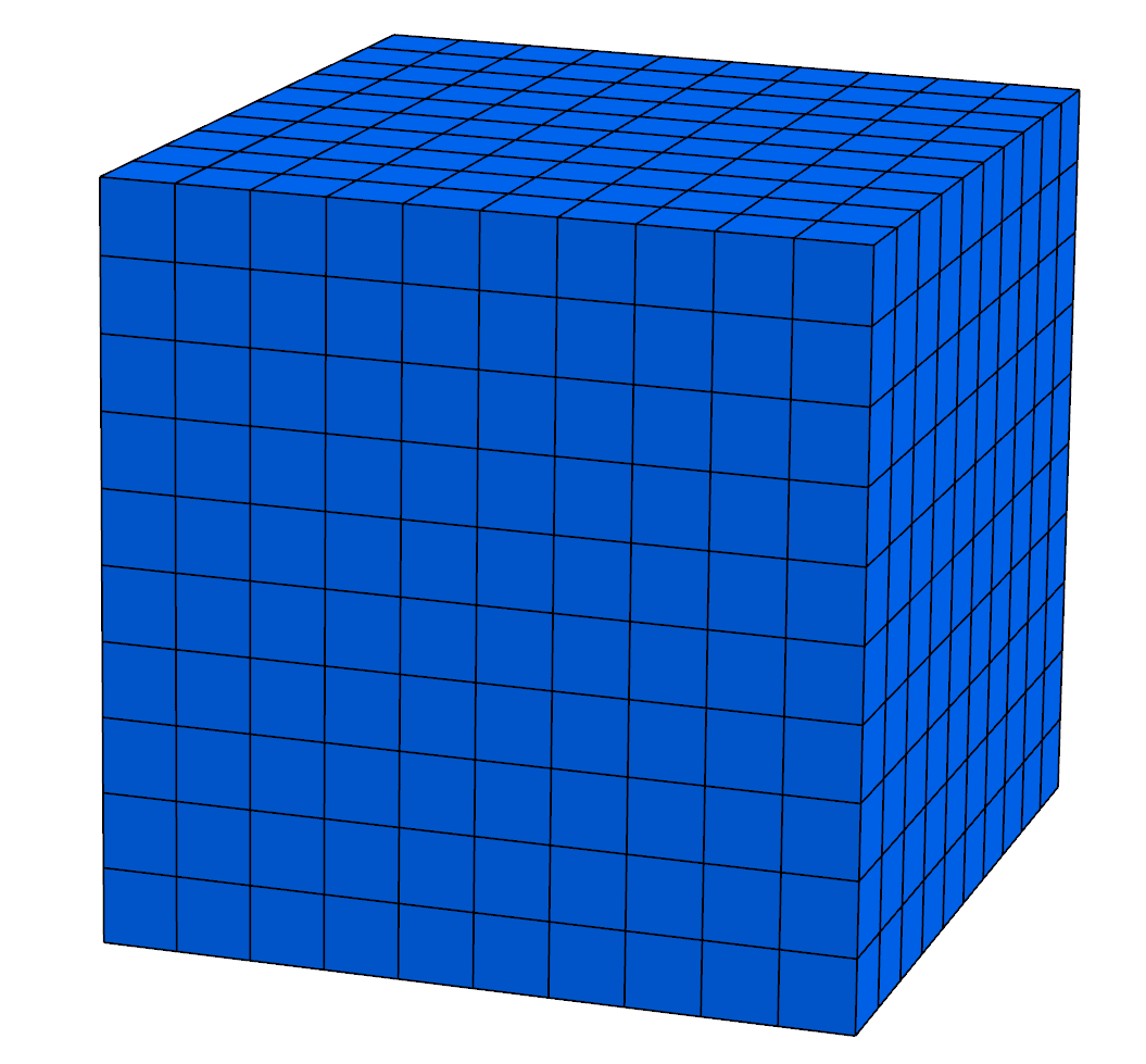
In this first part of the tutorial, we use a hexahedral mesh provided with GEOSX. This hexahedral mesh is strictly identical to the grid used in the first tutorial (Tutorial 1: First steps), but instead of using the internal grid generator GEOSX, we specify it with spatial node coordinates in MSH format.

The process by which grids are imported into GEOSX is worth explaining. To import external grid into GEOSX, we use an external component (submodule) called PAMELA. PAMELA (Parallel Meshing Library) was developed as a stand-alone utility to import grids in multiple formats and write them into memory for GEOSX. Although PAMELA is not necessary to run GEOSX (the internal grid generator of GEOSX has plenty of interesting features), you need PAMELA if you want to import external grids.

So here, our mesh consists of a simple sugar-cube stack of size 10x10x10. We inject fluid from one vertical face of a cube (the face corresponding to x=0), and we let the pressure equilibrate in the closed domain. The displacement is a single-phase, compressible fluid subject to gravity forces, so we expect the pressure to be constant on the injection face, and to be close to hydrostatic on the opposite plane (x=10). We use GEOSX to compute the pressure inside each grid block over a period of time of 100 seconds.

To see how to import such a mesh, we inspect the following XML file:

src/coreComponents/physicsSolvers/integratedTests/singlePhaseFlow/pamela_test/3D_10x10x10_compressible_pamela_hex_gravity.xml

In the XML Mesh tag, instead of an InternalMesh tag, we have a PAMELAMeshGenerator tag. We see that a file called cube_10x10x10_hex.msh is imported using PAMELA, and this object is instantiated with a user-defined name value. The file here contains geometric information in MSH format (it can also contain properties, as we will see in the next tutorial).

  <Mesh>
    <PAMELAMeshGenerator
      name="CubeHex"
      file="cube_10x10x10_hex.msh"/>
  </Mesh>

Here are the first few lines of the msh file :

Listing 1 cube_10x10x10_hex.msh¶

$MeshFormat
2 0 8
$EndMeshFormat
$Nodes
1331
0	0	0
10	0	0
10	10	0
0	10	0
0	0	10
10	0	10
10	10	10
0	10	10
1	0	0
2	0	0
3	0	0
4	0	0
5	0	0
6	0	0
7	0	0

GEOSX can run different physical solvers on different regions of the mesh at different times. Here, to keep things simple, we run one solver (single-phase flow) on the entire domain throughout the simulation. Even this is trivial, we need to define and name a region encompassing the entire domain and assign it to the single-phase flow solver. We also need to provide material properties to the regions. This is done by specifying ElementRegions. Here, the entire field is one region called Domain, and contains water and rock only.

  <ElementRegions>
    <CellElementRegion
      name="Domain"
      cellBlocks="{ DEFAULT_HEX }"
      materialList="{ water, rock }"/>
  </ElementRegions>

Running GEOSX¶

The command to run GEOSX is

path/to/geosx -i ../../../../coreComponents/physicsSolvers/fluidFlow/integratedTests/singlePhaseFlow/pamela_test/3D_10x10x10_compressible_pamela_hex_gravity.xml

Note that all paths for files included in the XML file are relative to this XML file, not to the GEOSX executable. When running GEOSX, console messages will provide indications regarding the status of the simulation.

In our case, the first lines are:

Adding Solver of type SinglePhaseFlow, named SinglePhaseFlow
Adding Mesh: PAMELAMeshGenerator, CubeHex
Adding Geometric Object: Box, all
Adding Geometric Object: Box, left
Adding Event: PeriodicEvent, solverApplications
Adding Event: PeriodicEvent, outputs
Adding Event: PeriodicEvent, restarts
Adding Output: Silo, siloWellPump
Adding Output: Restart, restartOutput
Adding Object CellElementRegion named Domain from ObjectManager::Catalog.

This indicates initialization of GEOSX. The mesh preprocessing tool PAMELA is launched next, with console messages as follows.

>>> **********************************************************************
>>>                          PAMELA Library Import tool
>>> **********************************************************************
>>> GMSH FORMAT IDENTIFIED
>>> *** Importing Gmsh mesh format...
>>> Reading nodes...
>>> Done0
>>> Reading elements...
>>> Number of nodes = 1331
>>> Number of triangles = 0
>>> Number of quadrilaterals = 0
>>> Number of tetrahedra = 0
>>> Number of hexahedra = 1000
>>> Number of pyramids = 0
>>> Number of prisms = 0
>>> *** Done
>>> *** Creating Polygons from Polyhedra...
>>> 3300 polygons have been created
>>> *** Done
>>> *** Perform partitioning...
>>> TRIVIAL partioning...
>>> Ghost elements...
>>> Clean mesh...
>>> *** Done...
>>> Clean Adjacency...
>>> *** Done...
Writing into the GEOSX mesh data structure
Running simulation

Notice the specification of the number of nodes (1331), and hexahedra (1000). After the adjacency calculations, GEOSX starts the simulation itself. with the time-step increments specified in the XML file.

At the end of your simulation, you should see something like:

Time: 99s, dt:1s, Cycle: 99
Cleaning up events
Writing out restart file at 3D_10x10x10_compressible_pamela_hex_gravity_restart_000000100/rank_0000000.hdf5

init time = 0.081181s, run time = 5.4595s

Once this is done, GEOSX is finished and we can inspect the outcome.

Visualization of results in VisIt¶

All results are written in a format compatible with VisIt. To load the results, point VisIt to the database file written in the Silo output folder.

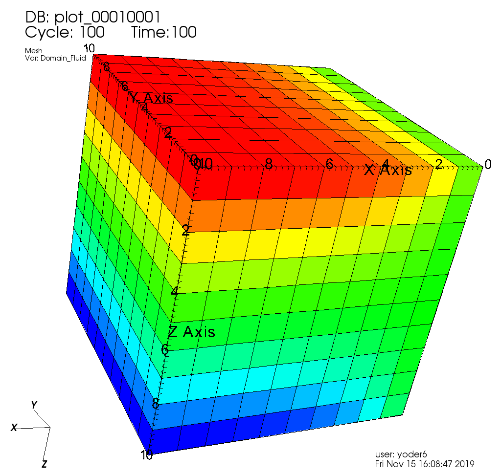
We see that the face x=0 shown here in the back of the illustration applies a constant pressure boundary condition (colored in green), whereas the face across from it displays a pressure field under gravity effect, equilibrated and hydrostatic. These results are consistent with what we expect.

Let us now see if a tetrahedral mesh, under the same exact physical conditions, can reproduce these results.

Externally Generated Tetrahedral Elements¶

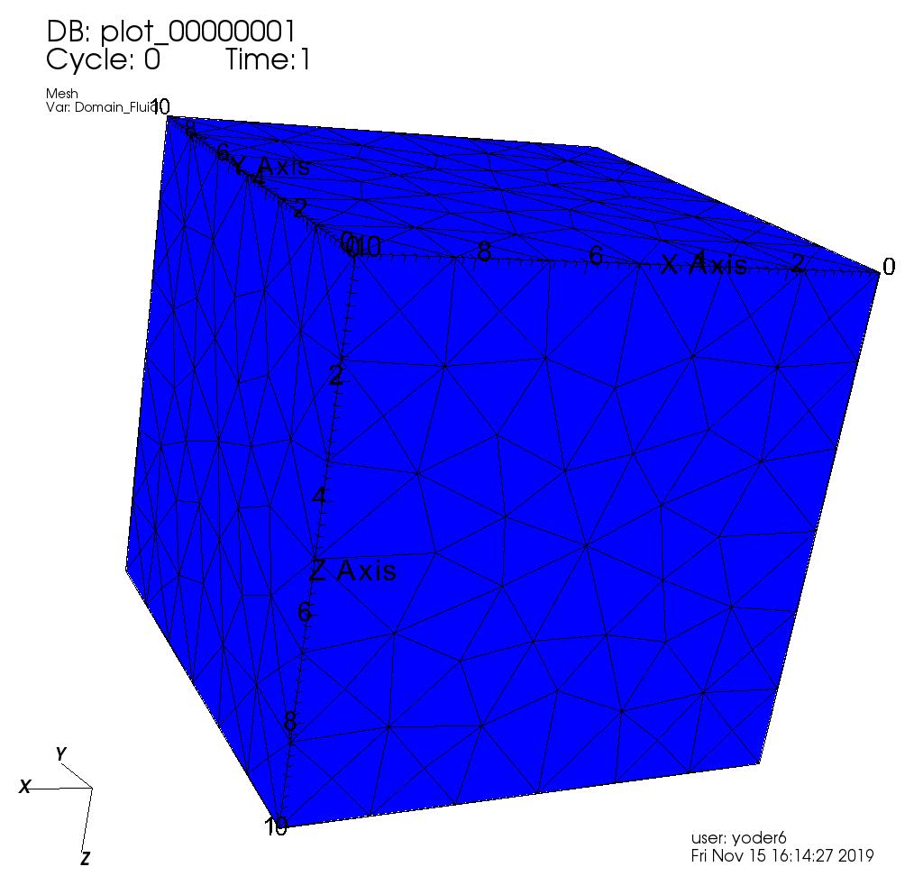
In the second part of the tutorial, we discretize the same cubic domain but with tetrahedral elements. Tetrahedral meshes are not yet common in geomodeling but offer tremendous flexibility in modeling fracture planes, faults, complex reservoir horizons and boundaries. Just like for hexahedral meshes, and for the same reasons (compatibility with finite volume and finite element methods), tetrahedral meshes in GEOSX must be conformal.

As stated previously, the problem we wish to solve here is the exact same physical problem as with hexahedral grid blocks. We apply a constant pressure condition (injection) from the x=0 vertical face of the domain, and we let pressure equilibrate over time. We observe the opposite side of the cube and expect to see hydrostatic pressure profiles because of the gravitational effect. The displacement is a single phase, compressible flow subject to gravity forces. We use GEOSX to compute the pressure inside each grid block.

The set-up for this problem is almost identical to the hexahedral mesh set-up. We simply point our Mesh tag to include a tetrahedral grid. The beauty of not relying on I,J,K indices for any property specification or well trajectory makes it easy to try different meshes for the same physical problems with GEOSX. Swapping out meshes without requiring other modifications to the input files makes mesh refinement studies easy to perform with GEOSX.

Like before, the XML file for this problem is the following:

src\CoreComponents\physicsSolvers\integratedTests\singlePhaseFlow\pamela_test\3D_10x10x10_compressible_pamela_tetra_gravity.xml

The only difference, is that now, the Mesh tag points GEOSX to a different mesh file called cube_10x10x10_tet.msh. This file contains nodes and tetrahedral elements in Gmsh format, representing a different discretization of the exact same 10x10x10 cubic domain.

  <Mesh>
    <PAMELAMeshGenerator
      name="CubeTetra"
      file="cube_10x10x10_tet.msh"/>
  </Mesh>

The mesh now looks like this:

And the MSH file starts as follows (notice the tetrahedral point coordinates as real numbers):

Listing 2 cube_10x10x10_tet.msh¶

$MeshFormat
2 0 8
$EndMeshFormat
$Nodes
366
0 0 10
0 0 0
0 10 10
0 10 0
10 0 10
10 0 0
10 10 10
10 10 0
0 0 1.666666666666662
0 0 3.333333333333323
0 0 4.999999999999986
0 0 6.666666666666647
0 0 8.333333333333321
0 1.666666666666662 10
0 3.333333333333323 10

Again, the entire field is one region called Domain and contains water and rock only.

  <ElementRegions>
    <CellElementRegion
      name="Domain"
      cellBlocks="{ DEFAULT_TETRA }"
      materialList="{ water, rock }"/>
  </ElementRegions>

Running GEOSX¶

The command to run GEOSX is

path/to/geosx -i ../../../../coreComponents/physicsSolvers/fluidFlow/integratedTests/singlePhaseFlow/pamela_test/cube_10x10x10_tet.msh

Again, all paths for files included in the XML file are relative to this XML file, not to the GEOSX executable. When running GEOSX, console messages will provide indications regarding the status of the simulation. In our case, the first lines are:

Adding Solver of type SinglePhaseFlow, named SinglePhaseFlow
Adding Mesh: PAMELAMeshGenerator, CubeTetra
Adding Geometric Object: Box, all
Adding Geometric Object: Box, left
Adding Event: PeriodicEvent, solverApplications
Adding Event: PeriodicEvent, outputs
Adding Event: PeriodicEvent, restarts
Adding Output: Silo, siloWellPump
Adding Output: Restart, restartOutput
Adding Object CellElementRegion named Domain from ObjectManager::Catalog.

Followed by:

>>> **********************************************************************
>>>                          PAMELA Library Import tool
>>> **********************************************************************
>>> GMSH FORMAT IDENTIFIED
>>> *** Importing Gmsh mesh format...
>>> Reading nodes...
>>> Done0
>>> Reading elements...
>>> Number of nodes = 366
>>> Number of triangles = 624
>>> Number of quadrilaterals = 0
>>> Number of tetrahedra = 1153
>>> Number of hexahedra = 0
>>> Number of pyramids = 0
>>> Number of prisms = 0
>>> *** Done
>>> *** Creating Polygons from Polyhedra...
>>> 1994 polygons have been created
>>> *** Done
>>> *** Perform partitioning...
>>> TRIVIAL partioning...
>>> Ghost elements...
>>> Clean mesh...
>>> *** Done...
>>> Clean Adjacency...
>>> *** Done...
Writing into the GEOSX mesh data structure

We see that we have now 366 nodes and 1153 tetrahedral elements. And finally, when the simulation is successfully done we see:

Running simulation
Time: 0s, dt:1s, Cycle: 0
Time: 1s, dt:1s, Cycle: 1
Time: 2s, dt:1s, Cycle: 2
Time: 3s, dt:1s, Cycle: 3
Time: 4s, dt:1s, Cycle: 4
Time: 5s, dt:1s, Cycle: 5
Time: 6s, dt:1s, Cycle: 6
...
Time: 96s, dt:1s, Cycle: 96
Time: 97s, dt:1s, Cycle: 97
Time: 98s, dt:1s, Cycle: 98
Time: 99s, dt:1s, Cycle: 99
Cleaning up events
Writing out restart file at 3D_10x10x10_compressible_pamela_tetra_gravity_restart_000000100/rank_0000000.hdf5

init time = 0.074377s, run time = 5.4331s

Visualization of results in VisIt¶

All results are written in a format compatible with VisIt by default. If we load into VisIt the .database file found in the Silo folder, we observe the following results:

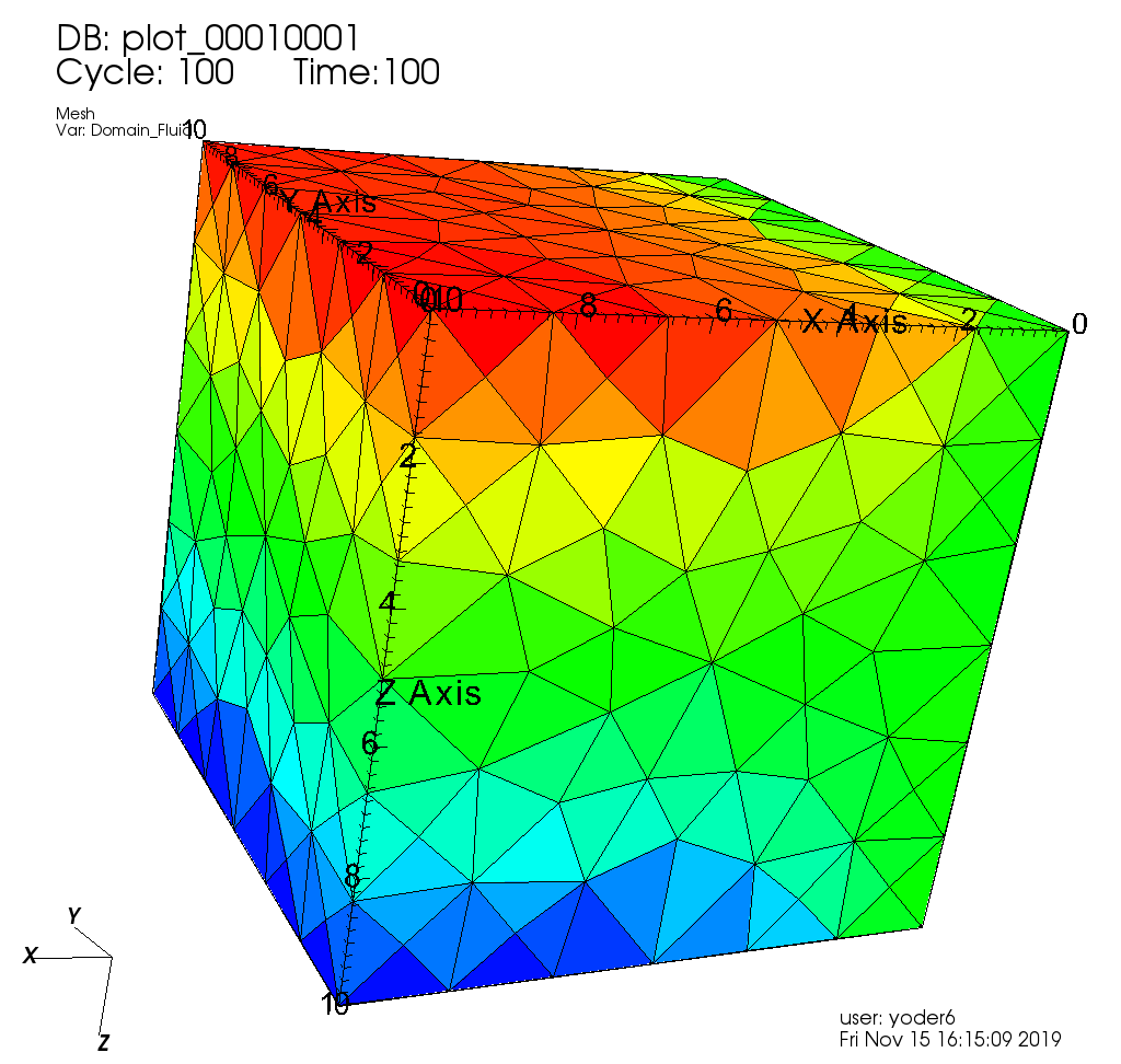
Here, we can see that despite the different mesh sizes and shapes, we are able to recover our pressure profile without any problems, or degradation in runtime performance.

To go further¶

Feedback on this tutorial

This concludes the single-phase external mesh tutorial. For any feedback on this tutorial, please submit a GitHub issue on the project’s GitHub page.

Next tutorial

In the next tutorial Tutorial 3: A simple field case, we learn how to run a simple field case with more complex unstructured meshes containing different regions and properties.

For more details

A complete description of the Internal Mesh generator is found here Meshes.

PAMELA being an external submodule has less documentation, but the same Meshes page may get you started.

GEOSX can handle tetrahedra, hexahedra, prisms, pyramids, wedges, and any combination thereof in one mesh. For more information on how MSH formats can help you specify these mesh types, see the Gmsh website.