Tutorial 3: A simple field case¶

Context

In this tutorial, we set up a simple field case for single-phase flow simulation (see Singlephase Flow Solver). We demonstrate how to run a basic flow simulation in the reservoir layer. We do not consider any coupling with wells. Injection and production will be specified by imposing a high pressure in the cells close to the injection area and a low pressure in the cells close to the production area.

Objectives

At the end of this tutorial you will know:

how to import external mesh information and properties,

how to run a specific solver (here, flow) in a specific region only,

the basic method of using boxes to set up boundary conditions,

how to use TableFunction to import fields varying in time and/or space,

how to control output frequency and export results for visualization.

Input file

The xml input file for this test case is located at:

src/coreComponents/physicsSolvers/multiphysics/integratedTests/FieldCaseTutorial1.xml

We consider the following mesh as a numerical support to the simulations in this tutorial:

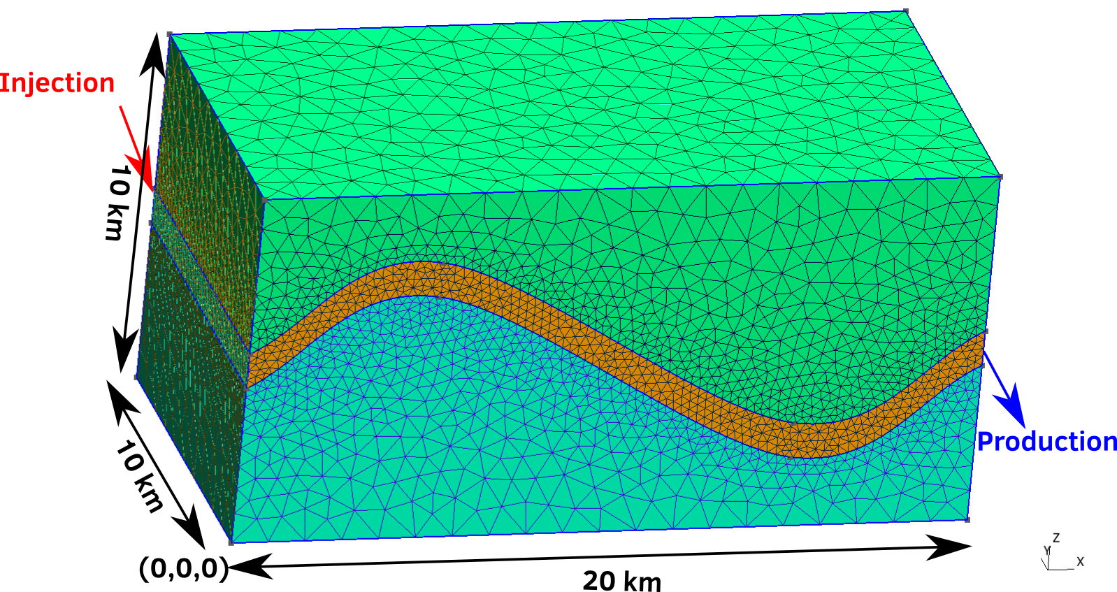
This mesh contains three continuous regions:

a Top region (overburden, elementary tag = Overburden)

a Middle region (reservoir layer, elementary tag = Reservoir)

a Bottom region (underburden, elementary tag = Underburden)

The mesh is defined using the GMSH file format (see Meshes for more information on the supported mesh file format). Each tetrahedron is associated to a unique tag.

GEOSX input files¶

The XML file considered here follows the typical structure of the GEOSX input files:

Solver

Mesh

Geometry

Events

NumericalMethods

ElementRegions

Constitutive

FieldSpecifications

Outputs

Functions

Defining a solver¶

Let us inspect the Solver XML tags.

  <Solvers
    gravityVector="0.0, 0.0, 0.0">
    <SinglePhaseFVM
      name="SinglePhaseFlow"
      logLevel="0"
      discretization="singlePhaseTPFA"
      fluidNames="{ water }"
      solidNames="{ rock }"
      targetRegions="{ Reservoir }">
      <NonlinearSolverParameters
        newtonTol="1.0e-6"
        newtonMaxIter="8"/>
      <LinearSolverParameters
        solverType="gmres"
        preconditionerType="amg"
        krylovTol="1.0e-10"/>
    </SinglePhaseFVM>
  </Solvers>

This node gathers all the information previously defined. We use a classical SinglePhaseFVM Finite Volume Method, with the two-point flux approximation as will be defined in the NumericalMethod tag. The targetRegions refers only to the Reservoir region because we only solve for flow in this region. The fluidNames and solidNames refer the materials defined in the Constitutive tag.

The NonlinearSolverParameters and LinearSolverParameters are used to set usual numerical solver parameters such as the linear and nonlinear tolerances, the preconditioner and solver types or the maximum number of nonlinear iterations.

Specifying a computational mesh¶

Here, we use the PAMELAMeshGenerator to load the mesh (see Importing the Mesh). The syntax to import external meshes is simple : in the XML file, the mesh file is included with its relative or absolute path to the location of the geosx XML file and a user-specified name label for the mesh object.

  <Mesh>
    <PAMELAMeshGenerator
      name="SyntheticMesh"
      file="synthetic.msh"/>
  </Mesh>

Geometry tag¶

Here, we are using definition of source and sink boxes in addition to the all box in order to flag sets of nodes or cells which will act as injection or production.

  <Geometry>
    <Box
      name="all"
      xMin="-1e9, -1e9, -1e9"
      xMax="1e9, 1e9, 1e9"/>

    <Box
      name="source"
      xMin="-0.1, 9700, 4499.9"
      xMax="300, 10000.01, 5500.1"/>

    <Box
      name="sink"
      xMin="19700, -0.1, 4499.9"
      xMax="20000.1, 300, 5500.1"/>
  </Geometry>

In order to define a box, the user defines xMax and xMin, two diagonally opposite nodes of the box.

Specifying events¶

The events are used here to guide the simulation through time, and specify when outputs must be triggered.

  <Events
    maxTime="500.0e6">
    <PeriodicEvent
      name="solverApplications"
      forceDt="2.0e6"
      target="/Solvers/SinglePhaseFlow"/>

    <PeriodicEvent
      name="outputs"
      timeFrequency="10.0e6"
      targetExactTimestep="1"
      target="/Outputs/syntheticReservoirVizFile"/>
  </Events>

The Events tag is associated with the maxTime keyword defining the maximum time. If this time is ever reached or exceeded, the simulation ends.

Two PeriodicEvent are defined. - The first one, solverApplications, is associated with the solver. The forceDt keyword means that there will always be time-steps of 23 days (2 000 000 seconds). - The second, outputs, is associated with the output. The timeFrequency keyword means that it will be executed every 116 days (10 000 000 seconds). The targetExactTimestep is set to 1, meaning that the Event Manager will impose this event will be triggered exactly every 116 days, constraining schedule decided by application to match this date.

Defining Numerical Methods¶

Defining the numerical method used in the solver, we will provide information on how to discretize our equations. Here a classical two-point flux approximation (TPFA) scheme is used to discretize water fluxes over faces.

  <NumericalMethods>
    <FiniteVolume>
      <TwoPointFluxApproximation
        name="singlePhaseTPFA"
        targetRegions="{ Reservoir }"
        fieldName="pressure"
        coefficientName="permeability"/>
    </FiniteVolume>
  </NumericalMethods>

The TwoPointFluxApproximation node should specify the primary field to solve for as fieldName. For a flow problem, this field is the pressure. Here we specified targetRegions as we only solve flow for reservoir. The field under coefficientName is used during TPFA transmissibilities construction.

Defining regions in the mesh¶

Assuming that the overburden and the underburden are impermeable, and flow only takes place in the reservoir, we need to define regions.

There are two methods to achieve this regional solve.

The first solution is to define a unique CellElementRegion corresponding to the reservoir.

<ElementRegion>
<CellElementRegion name="ReservoirLayer"
                   cellBlocks="{Reservoir_TETRA}"
                   materialList="{water, rock}">
</ElementRegion>

The second solution is to define all the CellElementRegions as they are in the GMSH file, but defining the solvers only on the reservoir layer. In this case, the ElementRegion tag is :

  <ElementRegions>
    <CellElementRegion
      name="Reservoir"
      cellBlocks="{ Reservoir_TETRA }"
      materialList="{ water, rock }"/>

    <CellElementRegion
      name="Burden"
      cellBlocks="{ Overburden_TETRA, Underburden_TETRA }"
      materialList="{ water, rock }"/>
  </ElementRegions>

We opt for the latest as it allows to visualize over- and underburdens and to change regions handling in ther tag without needing to amend the ElementRegion tag.

Note

The material list here was set for a single-phase flow problem. This list is subject to change if the problem is not a single-phase flow problem.

Defining material properties with constitutive laws¶

We simulate a single-phase flow in the reservoir layer, hence with two types of materials, a fluid (water) and solid (rock).

  <Constitutive>
    <CompressibleSinglePhaseFluid
      name="water"
      defaultDensity="1000"
      defaultViscosity="0.001"
      referencePressure="0.0"
      compressibility="1e-9"
      viscosibility="0.0"/>

    <PoreVolumeCompressibleSolid
      name="rock"
      referencePressure="0.0"
      compressibility="1e-9"/>
  </Constitutive>

The constitutive parameters such as the density, the viscosity, and the compressibility are specified in the International System of Units.

Note

To consider an incompressible fluid, the user has to set the compressibility to 0.

Defining properties with the FieldSpecifications¶

The next step is to specify fields, including:

The initial value (here, the pressure has to be initialized)

The static properties (here, we have to define the permeability tensor and the porosity)

The boundary conditions (here, the injection and production pressure have to be set)

  <FieldSpecifications>
    <FieldSpecification
      name="permx"
      initialCondition="1"
      component="0"
      setNames="{ all }"
      objectPath="ElementRegions/Reservoir/Reservoir_TETRA"
      fieldName="permeability"
      scale="1e-14"
      functionName="permxFunc"/>

    <FieldSpecification
      name="permy"
      initialCondition="1"
      component="1"
      setNames="{ all }"
      objectPath="ElementRegions/Reservoir/Reservoir_TETRA"
      fieldName="permeability"
      scale="1e-14"
      functionName="permyFunc"/>

    <FieldSpecification
      name="permz"
      initialCondition="1"
      component="2"
      setNames="{ all }"
      objectPath="ElementRegions/Reservoir/Reservoir_TETRA"
      fieldName="permeability"
      scale="1e-18"
      functionName="permzFunc"/>

    <FieldSpecification
      name="referencePorosity"
      initialCondition="1"
      setNames="{ all }"
      objectPath="ElementRegions/Reservoir/Reservoir_TETRA"
      fieldName="referencePorosity"
      scale="0.05"/>

    <FieldSpecification
      name="initialPressure"
      initialCondition="1"
      setNames="{ all }"
      objectPath="ElementRegions/Reservoir/Reservoir_TETRA"
      fieldName="pressure"
      scale="1"
      functionName="initialPressureFunc"/>

    <FieldSpecification
      name="sourceTerm"
      objectPath="ElementRegions/Reservoir/Reservoir_TETRA"
      fieldName="pressure"
      scale="1e7"
      setNames="{ source }"
      functionName="timeInj"/>

    <FieldSpecification
      name="sinkTerm"
      objectPath="ElementRegions/Reservoir/Reservoir_TETRA"
      fieldName="pressure"
      scale="0.0"
      setNames="{ sink }"/>
  </FieldSpecifications>

You may note :

All static parameters and initial value fields must have initialCondition field set to 1.

The objectPath refers to the ElementRegion in which the field has its value,

The setName field points to the box previously defined to apply the fields,

name and fieldName have a different meaning: name is used to give a name to the XML block. This name must be unique. fieldName is the name of the field registered in GEOSX. This value has to be set according to the expected input fields of each solver.

Note

GEOSX handles permeability as a diagonal matrix, so the three values of the permeability tensor are set individually using the component field,

Specifying the output formats¶

The Outputs XML tag is used to trigger the writing of visualization files. Here, we write files in a format natively readable by Paraview under the tar VTK

  <Outputs>
    <!--   <Silo name="syntheticReservoirVizFile"/> -->
    <VTK
      name="syntheticReservoirVizFile"/>
  </Outputs>

Note

The name keyword defines the name of the output directory.

Using Functions to specify dependent properties¶

Eventually, one can define varying properties using TableFunction (Functions) under the Functions tag:

  <Functions>
    <TableFunction
      name="timeInj"
      inputVarNames="{ time }"
      coordinates="{ 200e6, 250e6, 500e6 }"
      values="{ 1, 0.01, 0.00001 }"/>

    <TableFunction
      name="initialPressureFunc"
      inputVarNames="{ elementCenter }"
      coordinateFiles="{ tables_FieldCaseTuto/xlin.geos, tables_FieldCaseTuto/ylin.geos, tables_FieldCaseTuto/zlin.geos }"
      voxelFile="tables_FieldCaseTuto/pressure.geos"
      interpolation="linear"/>

    <TableFunction 
	name="permxFunc"
	inputVarNames="{elementCenter}"
	coordinateFiles="{tables_FieldCaseTuto/xlin.geos,tables_FieldCaseTuto/ylin.geos,tables_FieldCaseTuto/zlin.geos}"
	voxelFile="tables_FieldCaseTuto/permx.geos"
	interpolation="nearest" />

    <TableFunction 
	name="permyFunc"
	inputVarNames="{elementCenter}"
	coordinateFiles="{tables_FieldCaseTuto/xlin.geos,tables_FieldCaseTuto/ylin.geos,tables_FieldCaseTuto/zlin.geos}"
	voxelFile="tables_FieldCaseTuto/permy.geos"
	interpolation="nearest" />

    <TableFunction 
	name="permzFunc"
	inputVarNames="{elementCenter}"
	coordinateFiles="{tables_FieldCaseTuto/xlin.geos,tables_FieldCaseTuto/ylin.geos,tables_FieldCaseTuto/zlin.geos}"
	voxelFile="tables_FieldCaseTuto/permz.geos"
	interpolation="nearest" />
  </Functions>

Here, the injection pressure is set to vary with time. Attentive reader might have noticed that sourceTerm was bound to a TableFunction named timeInj under FieldSpecifications tag definition. The initial pressure is set based on the values contained in the table formed by the files which are specified. In particular, the files xlin.geos, ylin.geos and zlin.geos define a regular meshing of the bounding box containing the reservoir. The pressure.geos file then defines the values of the pressure at those points.

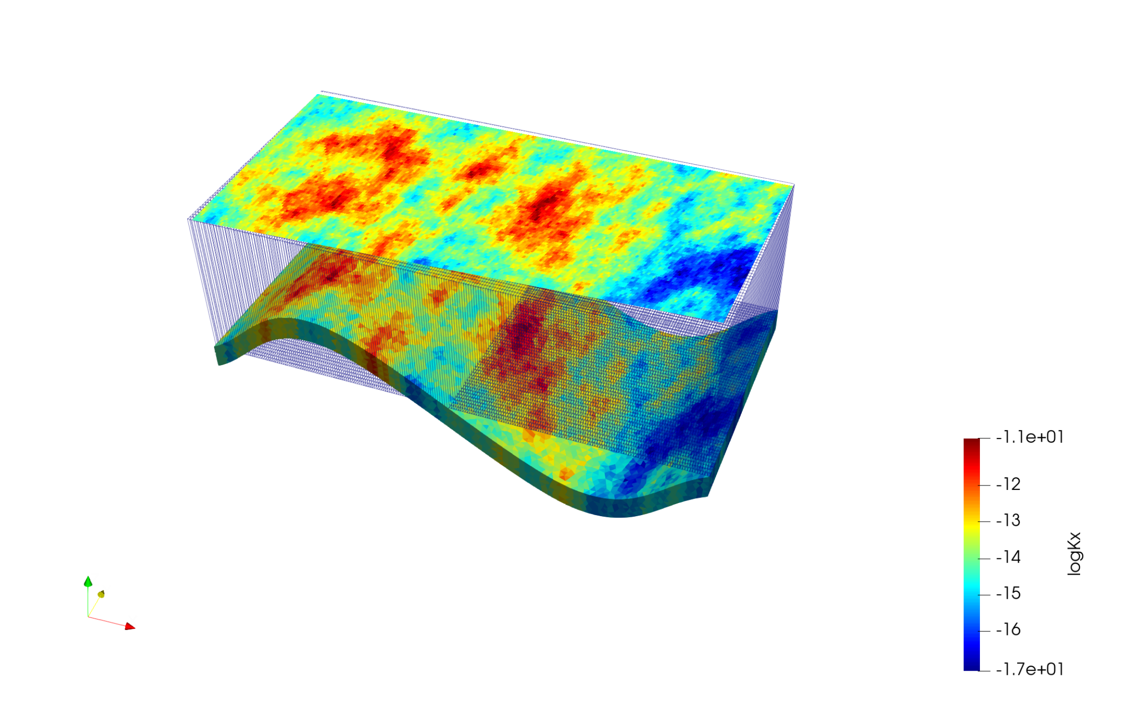
We proceed in a similar manner as for pressure.geos to map a heterogeneous permeability field (here the 5th layer of the SPE 10 test case) onto our unstructured grid. This mapping will use a nearest point interpolation rule.

Note

The varying values imposed in values or passed through voxelFile are premultiplied by the scale attribute from FieldSpecifications.

Running GEOSX¶

The simulation can be launched with:

geosx -i FieldCaseTutorial1.xml

One can notice the correct load of the field function among the starting output messages

Adding Mesh: PAMELAMeshGenerator, SyntheticMesh
Adding Solver of type SinglePhaseFVM, named SinglePhaseFlow
Adding Geometric Object: Box, all
Adding Geometric Object: Box, source
Adding Geometric Object: Box, sink
Adding Output: VTK, syntheticReservoirVizFile
Adding Event: PeriodicEvent, solverApplications
Adding Event: PeriodicEvent, outputs
   TableFunction: timeInj
   TableFunction: initialPressureFunc
   TableFunction: permxFunc
   TableFunction: permyFunc
   TableFunction: permzFunc
Adding Object CellElementRegion named Reservoir from ObjectManager::Catalog.
Adding Object CellElementRegion named Burden from ObjectManager::Catalog.

Visualization of results¶

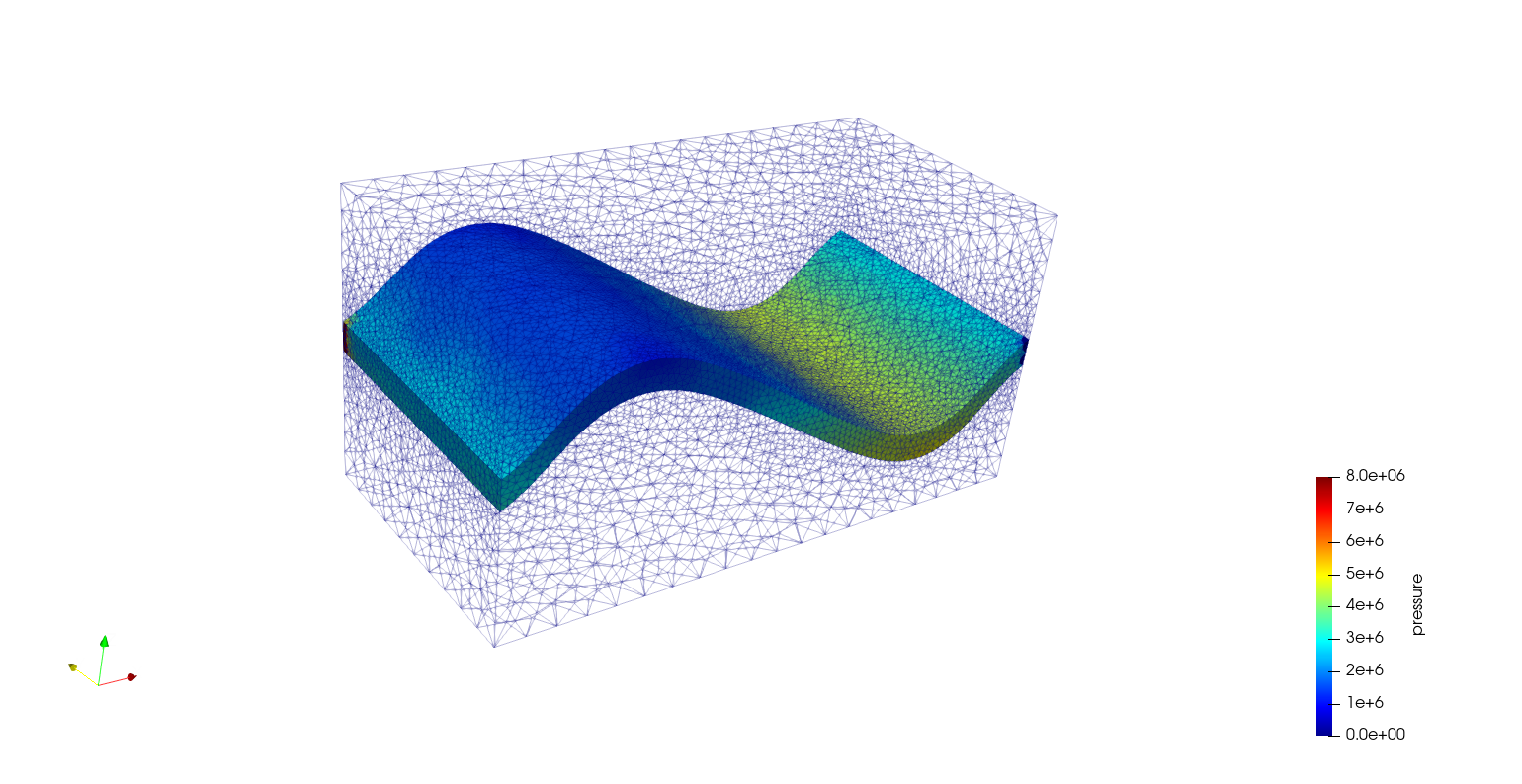
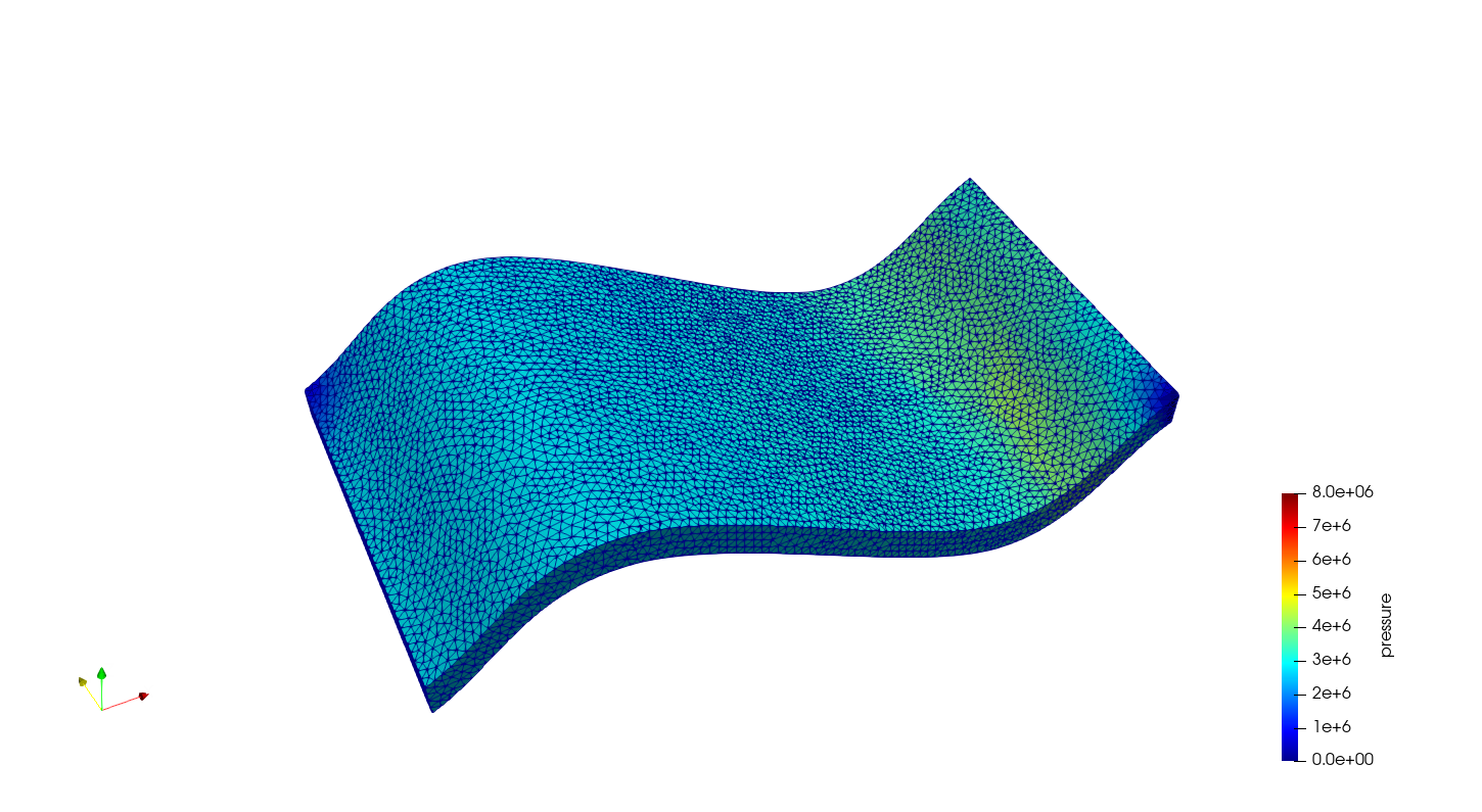
We can open the file syntheticReservoirVizFile.pvd with Paraview to visualize the simulation results. The initial pressure field in the reservoir region is provided below as an example.

../../../../_images/pressureField_initial.png

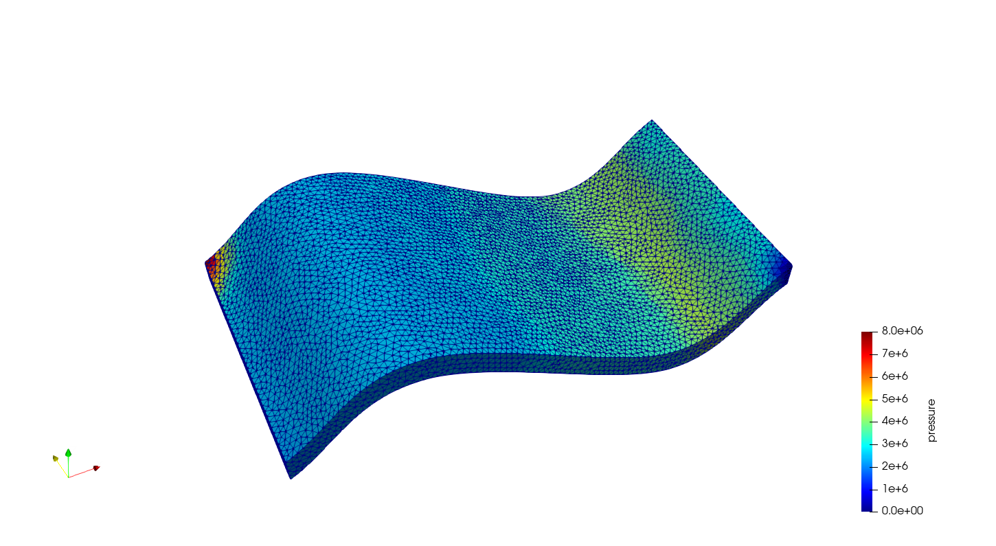
Since, in the event block, we have asked for the output to be generated at regular intervals throughout the simulation, we can also visualize the pressure distribution at different simulation times, showing the variation in the injection control.

../../../../_images/pressureField_2e8.png

../../../../_images/pressureField_5e8.png

To go further¶

Feedback on this tutorial

This concludes this tutorial. For any feedback, please submit a GitHub issue on the project’s GitHub page.

Next tutorial

In the next tutorial Tutorial 4: Multiphase flow with wells, we will learn how to run a dead oil case on a SPE10 channelized layer.

For more details

More on meshes, please see Meshes.

More on events, please see Event Management.