CO 2 Injection
Context
In this example, we show how to set up a multiphase simulation of CO 2 injection.
Objectives
At the end of this example you will know:
how to set up a CO 2 injection scenario with a well,
how to run a case using MPI-parallelism.
Input file
The XML file for this test case is located at :
inputFiles/compositionalMultiphaseWell/simpleCo2InjTutorial_base.xml
inputFiles/compositionalMultiphaseWell/simpleCo2InjTutorial_smoke.xml
This mesh is a simple internally generated regular grid (50 x 1 x 150). A single CO 2 injection well is at the center of the reservoir.
The XML file considered here follows the typical structure of the GEOS input files:
Multiphase flow and well solvers
Let us inspect the Solver XML tags. They consist of three blocks CompositionalMultiphaseFVM, CompositionalMultiphaseWell and CompositionalMultiphaseReservoir, which are respectively handling the solution from multiphase flow in the reservoir, multiphase flow in the wells, and coupling between those two parts.
  <Solvers>
    <CompositionalMultiphaseReservoir
      name="coupledFlowAndWells"
      flowSolverName="compositionalMultiphaseFlow"
      wellSolverName="compositionalMultiphaseWell"
      logLevel="1"
      initialDt="1e2"
      targetRegions="{ reservoir, wellRegion }">
      <NonlinearSolverParameters
        newtonTol="1.0e-4"
        lineSearchAction="None"
        maxTimeStepCuts="10"
        newtonMaxIter="40"/>
      <LinearSolverParameters
        solverType="fgmres"
        preconditionerType="mgr"
        krylovTol="1e-5"/>
    </CompositionalMultiphaseReservoir>

    <CompositionalMultiphaseFVM
      name="compositionalMultiphaseFlow"
      targetRegions="{ reservoir }"
      discretization="fluidTPFA"
      temperature="368.15"
      maxCompFractionChange="0.2"
      logLevel="1"
      useMass="1"/>

    <CompositionalMultiphaseWell
      name="compositionalMultiphaseWell"
      targetRegions="{ wellRegion }"
      maxCompFractionChange="0.2"
      logLevel="1"
      useMass="1">
      <WellControls
        name="wellControls"
        type="injector"
        control="totalVolRate"
        enableCrossflow="0"
        referenceElevation="6650"
        useSurfaceConditions="1"
        surfacePressure="101325"
        surfaceTemperature="288.71"
        targetBHP="5e7"
        targetTotalRate="1.5"
        injectionTemperature="368.15"
        injectionStream="{ 1, 0 }"/>
    </CompositionalMultiphaseWell>
  </Solvers>
In the CompositionalMultiphaseFVM (Compositional Multiphase Flow Solver), a classical multiphase compositional solver with a TPFA discretization is described.
The CompositionalMultiphaseWell (Compositional Multiphase Well Solver) consists of wellbore specifications (see Multiphase Flow with Wells for detailed example). As its reservoir counterpart, it includes references to fluid and relative permeability models, but also defines a WellControls sub-tag.
This sub-tag specifies the CO 2 injector control mode: the well is initially rate-controlled, with a rate specified in targetTotalRate and a maximum pressure specified in targetBHP. The injector-specific attribute, injectionStream, describes the composition of the injected mixture (here, pure CO 2).
The CompositionalMultiphaseReservoir coupling section describes the binding between those two previous elements (see Poromechanics for detailed example on coupling physics in GEOS). In addition to being bound to the previously described blocks through flowSolverName and wellSolverName sub-tags, it contains the initialDt starting time-step size value and defines the NonlinearSolverParameters and LinearSolverParameters that are used to control Newton-loop and linear solver behaviors (see Linear Solvers for a detailed description of linear solver attributes).
Note
To use the linear solver options of this example, you need to ensure that GEOS is configured to use the Hypre linear solver package.
Mesh and well geometry
In this example, the Mesh tag is used to generate the reservoir mesh internally (Tutorial 1: First Steps). The internal generation of well is defined with the InternalWell sub-tag. Apart from the name identifier attribute and their wellRegionName (ElementRegions) and wellControlsName (Solver) binding attributes, polylineNodeCoords and polylineSegmentConn attributes are used to define the path of the wellbore and connections between its nodes. The numElementsPerSegment discretizes the wellbore segments while the radius attribute specifies the wellbore radius (Multiphase Flow with Wells for details on wells). Once the wellbore is defined and discretized, the position of Perforations is defined using the linear distance from the head of the wellbore (distanceFromHead).
  <Mesh>
   <InternalMesh
      name="cartesianMesh"
      elementTypes="{ C3D8 }"
      xCoords="{ 0, 1000 }"
      yCoords="{ 450, 550 }"
      zCoords="{ 6500, 7700 }"
      nx="{ 50 }"
      ny="{ 1 }"
      nz="{ 150 }"
      cellBlockNames="{ cellBlock }">

      <InternalWell
        name="wellInjector1"
        wellRegionName="wellRegion"
        wellControlsName="wellControls"
        polylineNodeCoords="{ { 525.0, 525.0, 6650.00 },
                              { 525.0, 525.0, 6600.00 } }"
        polylineSegmentConn="{ { 0, 1 } }"
        radius="0.1"
        numElementsPerSegment="2">
        <Perforation
          name="injector1_perf1"
          distanceFromHead="45"/>
      </InternalWell>
   </InternalMesh>
  </Mesh>
Note
It is the responsibility of the user to make sure that there is a perforation in the bottom cell of the well mesh, otherwise an error will be thrown and the simulation will terminate.
Events
The solver is applied as a periodic event whose target is referred to as coupledFlowAndWells nametag.
Using the maxEventDt attribute, we specify a max time step size of 5 x  seconds.
The output event triggers a VTK output every  seconds, constraining the solver schedule to match exactly these dates.
The output path to data is specified as a
seconds, constraining the solver schedule to match exactly these dates.
The output path to data is specified as a target of this PeriodicEvent.
Another periodic event is defined under the name restarts.
It consists of saved checkpoints every 5 x seconds, whose physical output folder name is defined under the Output tag.
Finally, the time history collection and output events are used to trigger the mechanisms involved in the generation of a time series of well pressure (see the procedure outlined in Tasks Manager, and the example in Multiphase Flow with Wells).
  <Events
    maxTime="5e8">

    <PeriodicEvent
      name="outputs"
      timeFrequency="1e7"
      targetExactTimestep="1"
      target="/Outputs/simpleReservoirViz"/>

    <PeriodicEvent
      name="restarts"
      timeFrequency="5e7"
      targetExactTimestep="1"
      target="/Outputs/restartOutput"/>

    <PeriodicEvent
      name="timeHistoryCollection"
      timeFrequency="1e7"
      targetExactTimestep="1"
      target="/Tasks/wellPressureCollection" />

    <PeriodicEvent
      name="timeHistoryOutput"
      timeFrequency="2e8"
      targetExactTimestep="1"
      target="/Outputs/timeHistoryOutput" />

    <PeriodicEvent
      name="solverApplications"
      maxEventDt="5e5"
      target="/Solvers/coupledFlowAndWells"/>

  </Events>
Numerical methods
The TwoPointFluxApproximation is chosen for the fluid equation discretization. The tag specifies:
A primary field to solve for as
fieldName. For a flow problem, this field is pressure.A set of target regions in
targetRegions.A
coefficientNamepointing to the field used for TPFA transmissibilities construction.A
coefficientModelNamesused to specify the permeability constitutive model(s).
  <NumericalMethods>
    <FiniteVolume>
      <TwoPointFluxApproximation
        name="fluidTPFA"/>
    </FiniteVolume>
  </NumericalMethods>
Element regions
We define a CellElementRegion pointing to all reservoir mesh cells, and a WellElementRegion for the well. The two regions contain a list of constitutive model names. The keyword “all” is used here to automatically select all cells of the mesh.
  <ElementRegions>
    <CellElementRegion
      name="reservoir"
      cellBlocks="{ * }"
      materialList="{ fluid, rock, relperm }"/>

    <WellElementRegion
      name="wellRegion"
      materialList="{ fluid }"/>
  </ElementRegions>
Constitutive laws
Under the Constitutive tag, four items can be found:
CO2BrinePhillipsFluid : this tag defines phase names, component molar weights, and fluid behaviors such as CO 2 solubility in brine and viscosity/density dependencies on pressure and temperature.
PressurePorosity : this tag contains all the data needed to model rock compressibility.
BrooksCoreyRelativePermeability : this tag defines the relative permeability model for each phase, its end-point values, residual volume fractions (saturations), and the Corey exponents.
ConstantPermeability : this tag defines the permeability model that is set to a simple constant diagonal tensor, whose values are defined in
permeabilityComponent. Note that these values will be overwritten by the permeability field imported in FieldSpecifications.
  <Constitutive>
    <CO2BrinePhillipsFluid
      name="fluid"
      phaseNames="{ gas, water }"
      componentNames="{ co2, water }"
      componentMolarWeight="{ 44e-3, 18e-3 }"
      phasePVTParaFiles="{ pvtgas.txt, pvtliquid.txt }"
      flashModelParaFile="co2flash.txt"/>

    <CompressibleSolidConstantPermeability
      name="rock"
      solidModelName="nullSolid"
      porosityModelName="rockPorosity"
      permeabilityModelName="rockPerm"/>

    <NullModel
      name="nullSolid"/>

    <PressurePorosity
      name="rockPorosity"
      defaultReferencePorosity="0.05"
      referencePressure="1.0e7"
      compressibility="4.5e-10"/>

    <BrooksCoreyRelativePermeability
      name="relperm"
      phaseNames="{ gas, water }"
      phaseMinVolumeFraction="{ 0.05, 0.30 }"
      phaseRelPermExponent="{ 2.0, 2.0 }"
      phaseRelPermMaxValue="{ 1.0, 1.0 }"/>

    <ConstantPermeability
      name="rockPerm"
      permeabilityComponents="{ 1.0e-17, 1.0e-17, 3.0e-17 }"/>

  </Constitutive>
The PVT data specified by CO2BrinePhillipsFluid is set to model the behavior of the CO 2-brine system as a function of pressure, temperature, and salinity. We currently rely on a two-phase, two-component (CO 2 and H 2 O) model in which salinity is a constant parameter in space and in time. The model is described in detail in CO2-brine model. The model definition requires three text files:
In co2flash.txt, we define the CO 2 solubility model used to compute the amount of CO 2 dissolved in the brine phase as a function of pressure (in Pascal), temperature (in Kelvin), and salinity (in units of molality):
FlashModel CO2Solubility 1.0e5 7.5e7 1e5 285.15 395.15 5 0
The first keyword is an identifier for the model type (here, a flash model). It is followed by the model name. Then, the lower, upper, and step increment values for pressure and temperature ranges are specified. The trailing 0 defines a zero-salinity in the model. Note that the water component is not allowed to evaporate into the CO 2 -rich phase.
The pvtgas.txt and pvtliquid.txt files define the models used to compute the density and viscosity of the two phases, as follows:
DensityFun SpanWagnerCO2Density 1.0e5 7.5e7 1e5 285.15 395.15 5
ViscosityFun FenghourCO2Viscosity 1.0e5 7.5e7 1e5 285.15 395.15 5
DensityFun PhillipsBrineDensity 1.0e5 7.5e7 1e5 285.15 395.15 5 0
ViscosityFun PhillipsBrineViscosity 0
In these files, the first keyword of each line is an identifier for the model type (either a density or a viscosity model).
It is followed by the model name.
Then, the lower, upper, and step increment values for pressure and temperature ranges are specified.
The trailing 0 for PhillipsBrineDensity and PhillipsBrineViscosity entry is the salinity of the brine, set to zero.
Note
It is the responsibility of the user to make sure that the pressure and temperature values encountered in the simulation (in the reservoir and in the well) are within the bounds specified in the PVT files. GEOS will not throw an error if a value outside these bounds is encountered, but the (nonlinear) behavior of the simulation and the quality of the results will likely be negatively impacted.
Property specification
The FieldSpecifications tag is used to declare fields such as directional permeability, reference porosity, initial pressure, and compositions. Here, these fields are homogeneous, except for the permeability field that is taken as an heterogeneous log-normally distributed field and specified in Functions as in Tutorial 3: Regions and Property Specifications.
  <FieldSpecifications>
   <FieldSpecification
      name="permx"
      initialCondition="1"
      component="0"
      setNames="{ all }"
      objectPath="ElementRegions/reservoir"
      fieldName="rockPerm_permeability"
      scale="1e-15"
      functionName="permxFunc"/>

    <FieldSpecification
      name="permy"
      initialCondition="1"
      component="1"
      setNames="{ all }"
      objectPath="ElementRegions/reservoir"
      fieldName="rockPerm_permeability"
      scale="1e-15"
      functionName="permyFunc"/>

    <FieldSpecification
      name="permz"
      initialCondition="1"
      component="2"
      setNames="{ all }"
      objectPath="ElementRegions/reservoir"
      fieldName="rockPerm_permeability"
      scale="1.5e-15"
      functionName="permzFunc"/>

    <FieldSpecification
      name="initialPressure"
      initialCondition="1"
      setNames="{ all }"
      objectPath="ElementRegions/reservoir"
      fieldName="pressure"
      scale="1.25e7"/>

    <FieldSpecification
      name="initialComposition_co2"
      initialCondition="1"
      setNames="{ all }"
      objectPath="ElementRegions/reservoir"
      fieldName="globalCompFraction"
      component="0"
      scale="0.0"/>

    <FieldSpecification
      name="initialComposition_water"
      initialCondition="1"
      setNames="{ all }"
      objectPath="ElementRegions/reservoir"
      fieldName="globalCompFraction"
      component="1"
      scale="1.0"/>
  </FieldSpecifications>
Note
In this case, we are using the same permeability field (perm.geos) for all the directions. Note also that
the fieldName values are set to rockPerm_permeability to access the permeability field handled as
a Constitutive law. These permeability values will overwrite the values already set in the Constitutive block.
Warning
This XML file example does not take into account elevation when imposing the intial pressure with initialPressure.
Consider using a “HydrostraticEquilibrium” for a closer answer to modeled physical processes.
Output
The Outputs XML tag is used to write visualization, restart, and time history files.
Here, we write visualization files in a format natively readable by Paraview under the tag VTK. A Restart tag is also be specified. In conjunction with a PeriodicEvent, a restart file allows to resume computations from a set of checkpoints in time. Finally, we require an output of the well pressure history using the TimeHistory tag.
  <Outputs>
    <VTK
      name="simpleReservoirViz"/>

    <Restart
      name="restartOutput"/>

    <TimeHistory
      name="timeHistoryOutput"
      sources="{/Tasks/wellPressureCollection}"
      filename="wellPressureHistory" />

  </Outputs>
Tasks
In the Events block, we have defined an event requesting that a task periodically collects the pressure at the well.
This task is defined here, in the PackCollection XML sub-block of the Tasks block.
The task contains the path to the object on which the field to collect is registered (here, a WellElementSubRegion) and the name of the field (here, pressure).
The details of the history collection mechanism can be found in Tasks Manager.
  <Tasks>
    <PackCollection
      name="wellPressureCollection"
      objectPath="ElementRegions/wellRegion/wellRegionUniqueSubRegion"
      fieldName="pressure" />

  </Tasks>
Running GEOS
The simulation can be launched with 4 cores using MPI-parallelism:
mpirun -np 4 geosx -i simpleCo2InjTutorial_smoke.xml -x 2 -y 1 -z 2
A restart from a checkpoint file simpleCo2InjTutorial_restart_000000024.root is always available thanks to the following command line :
mpirun -np 4 geosx -i simpleCo2InjTutorial_smoke.xml -r simpleCo2InjTutorial_restart_000000024 -x 2 -y 1 -z 2
The output then shows the loading of HDF5 restart files by each core.
Loading restart file simpleCo2InjTutorial_restart_000000024
Rank 0: rankFilePattern = simpleCo2InjTutorial_restart_000000024/rank_%07d.hdf5
Rank 0: Reading in restart file at simpleCo2InjTutorial_restart_000000024/rank_0000000.hdf5
Rank 1: Reading in restart file at simpleCo2InjTutorial_restart_000000024/rank_0000001.hdf5
Rank 3: Reading in restart file at simpleCo2InjTutorial_restart_000000024/rank_0000003.hdf5
Rank 2: Reading in restart file at simpleCo2InjTutorial_restart_000000024/rank_0000002.hdf5
and the simulation restarts from this point in time.
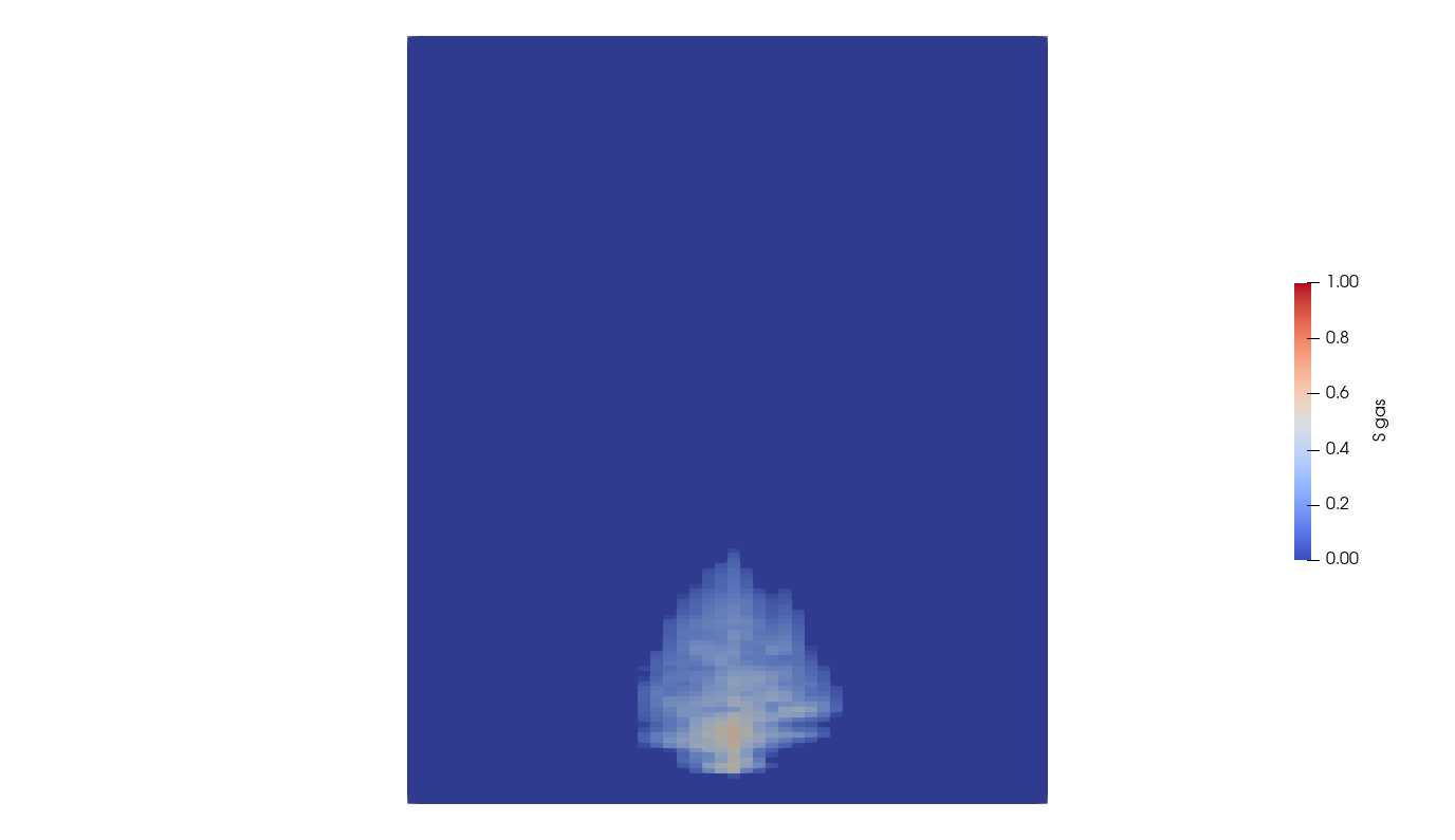
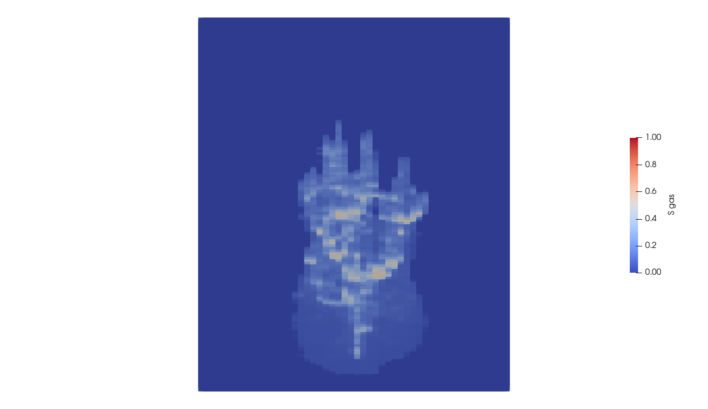
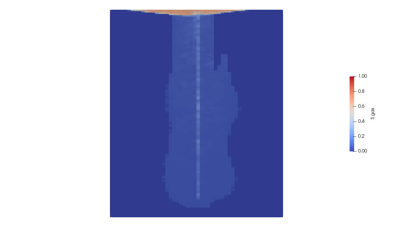
Visualization
Using Paraview, we can observe the CO 2 plume moving upward under buoyancy effects and forming a gas cap at the top of the domain,
The heterogeneous values of the permeability field can also be visualized in Paraview as shown below:
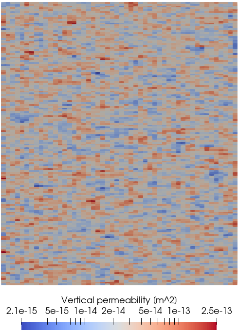
To go further
Feedback on this example
This concludes the CO 2 injection field case example. For any feedback on this example, please submit a GitHub issue on the project’s GitHub page.
For more details
A complete description of the reservoir flow solver is found here: Compositional Multiphase Flow Solver.
The well solver is described at Compositional Multiphase Well Solver.
The available fluid constitutive models are listed at Fluid Models.