Thermoporoelastic Consolidation

Context

Thermoporoelastic consolidation is a typical fully coupled problem which involves solid deformation, fluid flow and heat transfer in saturated porous media. In this example, we use the GEOS coupled solvers to solve a one-dimensional thermoporoelastic consolidation problem with a non-isothermal boundary condition, and we verify the accuracy of the results using the analytical solution provided in (Bai, 2005)

InputFile

This example uses no external input files and everything required is contained within two GEOS input files located at:

inputFiles/thermoPoromechanics/ThermoPoroElastic_consolidation_base.xml

inputFiles/thermoPoromechanics/ThermoPoroElastic_consolidation_benchmark_fim.xml

Description of the case

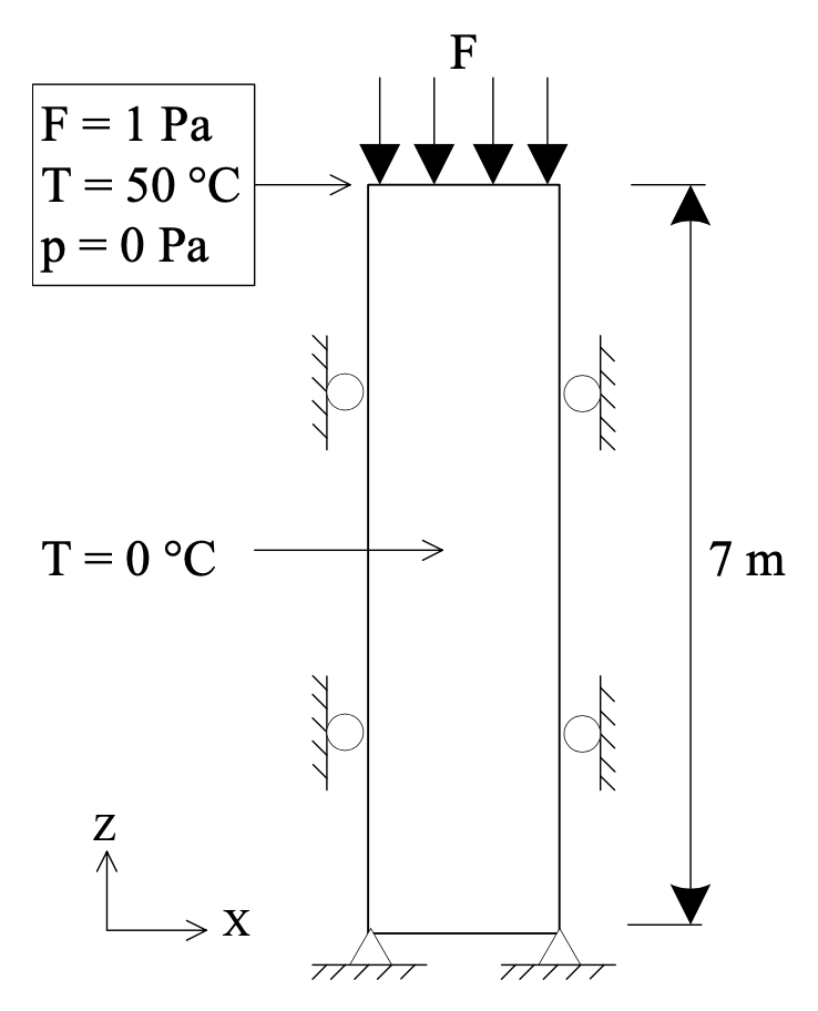
We simulate the consolidation of 1D thermoporoelastic column subjected to a surface traction stress of 1 Pa applied on the top surface, with a surface temperature of 50 degrees Celsius and a pore pressure of 0 Pa. The initial temperature of the saturated soil is 0 degrees Celsius. The soil column is insulated and sealed everywhere, except at the top surface. The problem setup is illustrated below.

../../../../../../_images/sketch5.png — Fig. 82 Sketch of the problem (taken from (Gao and Ghassemi, 2019)).

The coupled dynamics experienced by the system are described in (Gao and Ghassemi, 2019) and summarized below. The model first experiences continuous settlement (contraction). Initially, the settlement caused by the drainage of the fluid (effective stress increase) and the compression of the solid matrix is larger than the expansion due to the increase of temperature in the region close to the surface on which a higher temperature is applied. As the temperature diffuses further into the domain, it gradually rebounds (expansion) and reaches a final status.

For this example, we focus on the Solvers, the Constitutive, and the FieldSpecifications tags of the GEOS input file.

Solvers

As demonstrated in this example, to setup a thermoporomechanical coupling, we need to define three different solvers in the Solvers part of the XML file:

the mechanics solver, a solver of type SolidMechanicsLagrangianFEM called here solidMechSolver (more information here: Solid Mechanics Solver),

  <SolidMechanicsLagrangianFEM
    name="solidMechSolver"
    logLevel="1"
    discretization="FE1"
    targetRegions="{ Domain }"/>

the single-phase flow solver, a solver of type SinglePhaseFVM called here flowSolver (more information on these solvers at Singlephase Flow Solver),

  <SinglePhaseFVM
    name="flowSolver"
    logLevel="1"
    discretization="tpfaFlow"
    temperature="273.0"
    isThermal="1"
    targetRegions="{ Domain }">
    <NonlinearSolverParameters
      newtonMaxIter="100"
      newtonMinIter="0"
      newtonTol="1.0e-6"/>
    <LinearSolverParameters
      directParallel="0"/>
  </SinglePhaseFVM>

the coupling solver (SinglePhasePoromechanics) that will bind the two single-physics solvers above, which is named as thermoPoroSolver (more information at Poromechanics Solver).

  <SinglePhasePoromechanics
    name="thermoPoroSolver"
    solidSolverName="solidMechSolver"
    flowSolverName="flowSolver"
    isThermal="1"
    logLevel="1"
    targetRegions="{ Domain }">
    <NonlinearSolverParameters
      couplingType="FullyImplicit"
      newtonMaxIter="200"/>
    <LinearSolverParameters
      directParallel="0"/>
  </SinglePhasePoromechanics>

To request the simulation of the temperature evolution, we set the isThermal flag of the coupling solver to 1. With this choice, the degrees of freedom are the cell-centered pressure, the cell-centered temperature, and the mechanical displacements at the mesh nodes. The governing equations consist of a mass conservation equation, an energy balance equation, and a linear momentum balance equation. In the latter, the total stress includes both a pore pressure and a temperature contribution. Note that in the coupling solver, we set the couplingType to FullyImplicit to require a fully coupled, fully implicit solution strategy.

Constitutive laws

A homogeneous and isotropic domain with one solid material is assumed, and its mechanical properties and associated fluid rheology are specified in the Constitutive section. We use the constitutive parameters specified in (Bai, 2005) listed in the following table.

Symbol	Parameter	Unit	Value
$E$	Young’s modulus	[Pa]	6000.0
$\nu$	Poisson’s ratio	[-]	0.4
$\alpha$	Thermal expansion coef.	[T^(-1)]	9.0x10^-7
$\phi$	Porosity	[-]	0.20
$b$	Biot’s coefficient	[-]	1.0
$\rho C$	Heat capacity	[J/(m^3.K)]	167.2x10³
$\mu$	Fluid viscosity	[Pa.s]	1^-3
$k^T$	Thermal conductivity	[J/(m.s.K)]	836
$k$	Permeability	[m^2]	4.0x10^-9

The bulk modulus, the Young’s modulus, and the thermal expansion coefficient are specified in the ElasticIsotropic solid model. Note that for now the solid density is constant and does not depend on temperature. Given that the gravity vector has been set to 0 in the XML file, the value of the solid density is not used in this simulation.

    <ElasticIsotropic
      name="rockSolid"
      defaultDensity="2400"
      defaultBulkModulus="1e4"
      defaultShearModulus="2.143e3"
      defaultDrainedLinearTEC="3e-7"/>

The porosity and Biot’s coefficient (computed from the grainBulkModulus) appear in the BiotPorosity model. In this model, the porosity is updated as a function of the strain increment, the change in pore pressure, and the change in temperature.

    <BiotPorosity
      name="rockPorosity"
      defaultGrainBulkModulus="1.0e27"
      defaultReferencePorosity="0.2"
      defaultPorosityTEC="3e-7"/>

The heat capacity is provided in the SolidInternalEnergy model. In the computation of the internal energy, the referenceTemperature is set to the initial temperature.

    <SolidInternalEnergy
      name="rockInternalEnergy"
      referenceVolumetricHeatCapacity="1.672e5"
      referenceTemperature="0.0"
      referenceInternalEnergy="0.0"/>

The fluid density and viscosity are given in the ThermalCompressibleSinglePhaseFluid. Here, they are assumed to be constant and do not depend on pressure and temperature.

    <ThermalCompressibleSinglePhaseFluid
      name="water"
      defaultDensity="1000"
      defaultViscosity="1e-3"
      referencePressure="0.0"
      referenceTemperature="0.0"
      compressibility="0.0"
      thermalExpansionCoeff="0.0"
      viscosibility="0.0"
      specificHeatCapacity="1.672e2"
      referenceInternalEnergy="0.001"/>

Finally, the permeability and thermal conductivity are specified in the ConstantPermeability and SinglePhaseConstantThermalConductivity, respectively.

    <ConstantPermeability
      name="rockPerm"
      permeabilityComponents="{ 4.0e-9, 4.0e-9, 4.0e-9 }"/>
    
    <SinglePhaseThermalConductivity
      name="thermalCond"
      defaultThermalConductivityComponents="{ 836, 836, 836 }"/>

Initial and boundary conditions

To complete the specification of the problem, we specify two types of fields:

The initial values (the displacements, effective stress, and pore pressure have to be initialized),

The boundary conditions at the top surface (traction, pressure, and temperature) and at the other boundaries (zero-displacement).

This is done in the FieldSpecifications part of the XML file. The attribute initialCondition is set to 1 for the blocks specifying the initial pressure, temperature, and effective stress.

    <FieldSpecification
      name="initialPressure"
      initialCondition="1"
      setNames="{ all }"
      objectPath="ElementRegions/Domain/cb1"
      fieldName="pressure"
      scale="0.0"/>

    <FieldSpecification
      name="initialTemperature"
      initialCondition="1"
      setNames="{ all }"
      objectPath="ElementRegions/Domain/cb1"
      fieldName="temperature"
      scale="273.0"/>

    <FieldSpecification
      name="initialSigma_x"
      initialCondition="1"
      setNames="{ all }"
      objectPath="ElementRegions/Domain/cb1"
      fieldName="rockSolid_stress"
      component="0"
      scale="0.0"/>
    <FieldSpecification
      name="initialSigma_y"
      initialCondition="1"
      setNames="{ all }"
      objectPath="ElementRegions/Domain/cb1"
      fieldName="rockSolid_stress"
      component="1"
      scale="0.0"/>
    <FieldSpecification
      name="initialSigma_z"
      initialCondition="1"
      setNames="{ all }"
      objectPath="ElementRegions/Domain/cb1"
      fieldName="rockSolid_stress"
      component="2"
      scale="0.0"/>

For the zero-displacement boundary conditions, we use the pre-defined set names xneg and xpos, yneg, zneg and zpos to select the boundary nodes. Note that here, we have considered a slab in the y-direction, which is why a displacement boundary condition is applied on zpos and not applied on ypos.

    <FieldSpecification
      name="xconstraint"
      fieldName="totalDisplacement"
      component="0"
      objectPath="nodeManager"
      setNames="{ xneg, xpos }"/>

    <FieldSpecification
      name="yconstraint"
      fieldName="totalDisplacement"
      component="1"
      objectPath="nodeManager"
      setNames="{ yneg }"/>

    <FieldSpecification
      name="zconstraint"
      fieldName="totalDisplacement"
      component="2"
      objectPath="nodeManager"
      setNames="{ zneg, zpos }"/>

On the top surface, we impose the traction boundary condition and the non-isothermal boundary condition specified in (Bai, 2005). We also fix the pore pressure to 0 Pa.

    <Traction
      name="traction"
      objectPath="faceManager"
      tractionType="normal"
      scale="-1.0"
      setNames="{ ypos }"
      functionName="timeFunction"/>

    <FieldSpecification
      name="boundaryPressure"
      objectPath="faceManager"
      fieldName="pressure"
      scale="0.0"
      setNames="{ ypos }"/>

    <FieldSpecification
      name="boundaryTemperature"
      objectPath="faceManager"
      fieldName="temperature"
      scale="323.0"
      setNames="{ ypos }"/>

Inspecting results

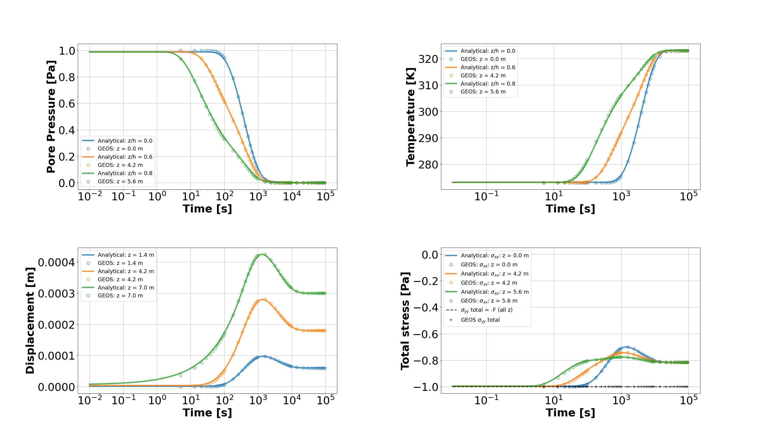
We request an output of the displacements, pressure, temperature, and stress using the TimeHistory feature of GEOS. The figure below compares the results from GEOS (open circles) with the corresponding analytical solution (solid lines) as a function of time at different locations along the slab. We obtain a very good match for all four quantities, confirming that GEOS accurately captures the thermo-poromechanical coupling on this example.

The top-left panel shows the excellent agreement for the pore pressure evolution: the initial thermally- and mechanically-induced overpressure gradually dissipates as the fluid drains through the top surface.

The top-right panel confirms the good match for the temperature, which diffuses from the heated top boundary into the column.

The bottom-left panel shows that GEOS also reproduces the vertical displacement (settlement), including the characteristic non-monotonic response (thermal expansion followed by consolidation).

The bottom-right panel compares the total stress. By equilibrium, the total vertical stress remains equal to the applied surface load at all times and depths ( $\sigma_{yy} = -F$ ), which GEOS recovers exactly. The total horizontal stress $\sigma_{xx} = \sigma_{zz}$ follows the uniaxial-strain thermo-poroelastic relation $\sigma_{xx} = -(\lambda/M)\,F - (2G/M)\,(3K\alpha_s\,\Delta T + b\,p)$ (with $M = K + 4G/3$ the oedometric modulus), exhibiting the transient overshoot driven by the coupled pressure and thermal fields.

(Source code)

To go further

Feedback on this example

For any feedback on this example, please submit a GitHub issue on the project’s GitHub page.