Model Initialization: Hydrostatic and Mechanical Equilibrium
Context
Prior to simulating underground operations, it is necessary to run a few steps of a fully coupled geomechanical simulation to reach the equilibrium state. In this example, we perform a gravity-only stress initialization for a reservoir with a hydrostatic in-situ pressure. The problem is solved using a single-phase poromechanics solver (see Poromechanics Solver) and the HydrostaticEquilibrium initialization procedure (see Hydrostatic Equilibrium Initial Condition) in GEOS to predict the initial state of stress with depth in the reservoir, subject to the reservoir rock properties and the prevailing hydrostatic pressure condition. This way, the poromechanical model is initialized at mechanical equilibrium and all displacements are set to zero after initialization. We verify numerical results obtained by GEOS against an analytical equation (Eaton’s equation).
Input file
The xml input files for the test case are located at:
inputFiles/initialization/gravityInducedStress_initialization_base.xml
inputFiles/initialization/gravityInducedStress_initialization_benchmark.xml
A Python script for post-processing the simulation results is provided:
src/coreComponents/physicsSolvers/multiphysics/docs/gravityInducedStressInitialization/gravityInitializationFigure.py
Description of the Case
We model the in-situ state of stress of a subsurface reservoir subject to a gravity-only induced stress and hydrostatic in-situ pressure condition. The domain is homogenous, isotropic and isothermal. The domain is subject to roller boundary conditions on lateral surfaces and at the base of the model, while the top of the model is a free surface.
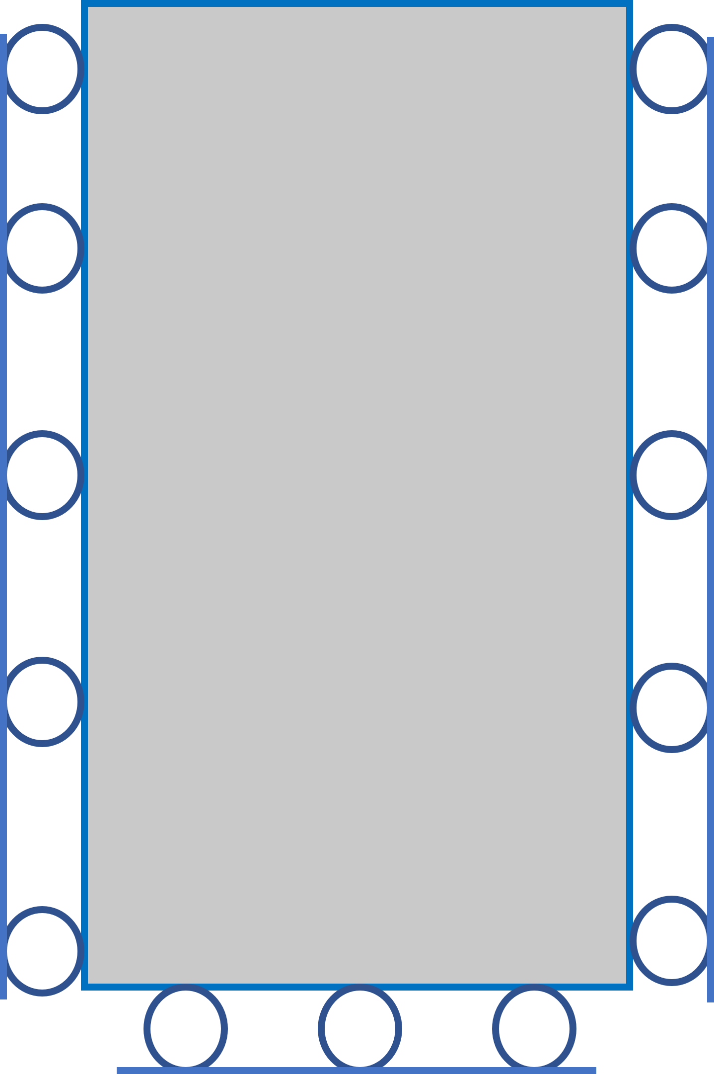
Fig. 92 Sketch of the problem
We set up and solve a PoroMechanics model to obtain the gradient of total stresses (principal stress components) across the domain due to gravity effects and hydrostatic pressure only. These numerical predictions are compared with the analytical solutions derived from Eaton et al. (1969, 1975)
For this example, we focus on the Mesh,
the Constitutive, and the FieldSpecifications tags.
Mesh
The following figure shows the mesh used for solving this poromechanical problem:
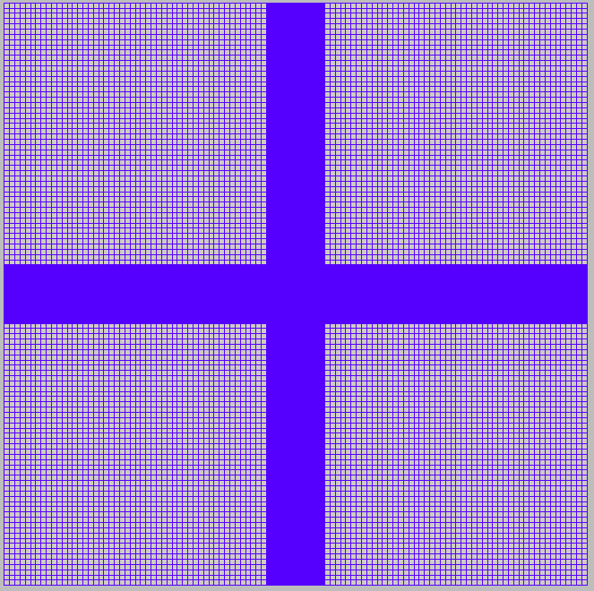
Fig. 93 Generated mesh
The mesh was created with the internal mesh generator and parametrized in the InternalMesh XML tag.
It contains 20x20x40 eight-node brick elements in the x, y, and z directions respectively.
Such eight-node hexahedral elements are defined as C3D8 elementTypes, and their collection forms a mesh
with one group of cell blocks named here cellBlockNames.
  <Mesh>
    <InternalMesh
      name="mesh1"
      elementTypes="{ C3D8 }"
      xCoords="{ 0.0, 1000 }"
      yCoords="{ 0.0, 1000 }"
      zCoords="{ -1000, 0 }"
      nx="{ 20 }"
      ny="{ 20 }"
      nz="{ 40 }"
      cellBlockNames="{ cb1 }" />
  </Mesh>
Poro-Mechanics Solver
For the initialization test, a hydrostatic pore pressure is imposed on the system. This is done using the Hydrostatic Equilibrium tag under Field Specifications. We then define a poro-mechanics solver called here poroSolve.
This solid mechanics solver (see Solid Mechanics Solver) called lagSolve is based on the Lagrangian finite element formulation.
The problem is run as QuasiStatic without considering inertial effects.
The computational domain is discretized by FE1, defined in the NumericalMethods section.
We use the targetRegions attribute to define the regions where the poromechanics solver is applied.
Since we only have one cellBlockName type called Domain, the poromechanics solver is applied to every element of the model.
The flow solver for this problem (see Singlephase Flow Solver) called SinglePhaseFlow is discretized by fluidTPFA, defined in the NumericalMethods section.
    <SinglePhasePoromechanics
      name="poroSolve"
      solidSolverName="lagsolve"
      flowSolverName="SinglePhaseFlow"
      logLevel="1"
      targetRegions="{ Domain }">
      <NonlinearSolverParameters
        newtonMaxIter="2"
        newtonTol="1.0e-2"
        maxTimeStepCuts="1"
        lineSearchMaxCuts="0" />
      <LinearSolverParameters
        directParallel="0" />
    </SinglePhasePoromechanics>
  <NumericalMethods>
    <FiniteElements>
      <FiniteElementSpace
        name="FE1"
        order="1" />
    </FiniteElements>

    <FiniteVolume>
      <TwoPointFluxApproximation
        name="fluidTPFA" />
    </FiniteVolume>
  </NumericalMethods>
Constitutive Laws
A homogeneous domain with one solid material is assumed, and its mechanical and fluid properties are specified in the Constitutive section:
  <Constitutive>
    <PorousElasticIsotropic
      name="rock"
      solidModelName="rockSolid"
      porosityModelName="rockPorosity"
      permeabilityModelName="rockPerm" />

    <ElasticIsotropic
      name="rockSolid"
      defaultDensity="2500"
      defaultPoissonRatio="0.25"
      defaultYoungModulus="100.0e6" />

    <BiotPorosity
      name="rockPorosity"
      defaultGrainBulkModulus="1.0e27"
      defaultReferencePorosity="0.375" />

    <ConstantPermeability
      name="rockPerm"
      permeabilityComponents="{ 1.0e-12, 1.0e-12, 1.0e-12 }" />

    <CompressibleSinglePhaseFluid
      name="water"
      defaultDensity="1000"
      defaultViscosity="0.001"
      referencePressure="0.000"
      referenceDensity="1000"
      compressibility="4.4e-10"
      referenceViscosity="0.001"
      viscosibility="0.0" />
  </Constitutive>
As shown above, in the CellElementRegion section,
rock is the solid material in the computational domain and water is the fluid material.
Here, Porous Elastic Isotropic model PorousElasticIsotropic is used to simulate the elastic behavior of rock.
As for the solid material parameters, defaultDensity, defaultPoissonRatio, defaultYoungModulus, grainBulkModulus, defaultReferencePorosity, and permeabilityComponents denote the rock density, Poisson ratio, Young modulus, grain bulk modulus, porosity, and permeability components respectively. In additon, the fluid property (water) of density, viscosity, compressibility and viscosibility are specified with defaultDensity, defaultViscosity, compressibility, and viscosibility.
All properties are specified in the International System of Units.
Stress Initialization Function
In the Tasks section, SinglePhasePoromechanicsInitialization tasks are defined to initialize the model by calling the poro-mechanics solver poroSolve. This task is used to determine stress gradients through designated densities and established constitutive relationships to maintain mechanical equilibrium and reset all initial displacements to zero following the initialization process.
  <Tasks>
    <SinglePhasePoromechanicsInitialization
      logLevel="1"
      name="singlephasePoromechanicsPreEquilibrationStep"
      poromechanicsSolverName="poroSolve" />
  </Tasks>
The initialization is triggered into action using the Event management section, where the soloEvent function calls the task at the target time (in this case -1e10s).
  <Events
    maxTime="10.0"
    minTime="-1e10">

    <PeriodicEvent
      name="outputs"
      timeFrequency="10.0"
      target="/Outputs/vtkOutput" />

    <PeriodicEvent
      name="solverApplication0"
      beginTime="0.0"
      endTime="10.0"
      target="/Solvers/poroSolve" />

    <SoloEvent
      beginTime="-1e10"
      name="singlephasePoromechanicsPreEquilibrationStep"
      target="/Tasks/singlephasePoromechanicsPreEquilibrationStep"
      targetTime="-1e10" />

  </Events>
The PeriodicEvent function is used here to define recurring tasks that progress for a stipulated time during the simuation. We also use it in this example to save the vtkOuput results.
  <Outputs>
    <VTK
      name="vtkOutput" />

    <Restart
      name="restartOutput"/>
  </Outputs>
We use Paraview to extract the data from the vtkOutput files at the initialization time, and then use a Python script to read and plot the stress and pressure gradients for verification and visualization.
Initial and Boundary Conditions
The next step is to specify fields, including:
The initial value (hydrostatic equilibrium),
The boundary conditions (the displacement control of the outer boundaries have to be set).
In this problem, all outer boundaries of the domain are subject to roller constraints except the top of the model, left as a free surface.
These boundary conditions are set up through the FieldSpecifications section.
  <FieldSpecifications>
    <HydrostaticEquilibrium
      datumElevation="0.0"
      datumPressure="0.0"
      name="equil"
      objectPath="ElementRegions/Domain" />

    <FieldSpecification
      name="xconstraint"
      objectPath="nodeManager"
      fieldName="totalDisplacement"
      component="0"
      scale="0.0"
      setNames="{ xneg, xpos }" />

    <FieldSpecification
      name="yconstraint"
      objectPath="nodeManager"
      fieldName="totalDisplacement"
      component="1"
      scale="0.0"
      setNames="{ yneg, ypos }" />

    <FieldSpecification
      name="zconstraint"
      objectPath="nodeManager"
      fieldName="totalDisplacement"
      component="2"
      scale="0.0"
      setNames="{ zneg }" />

  </FieldSpecifications>
The parameters used in the simulation are summarized in the following table.
Symbol |
Parameter |
Unit |
Value |
|---|---|---|---|
|
Young Modulus |
[MPa] |
100 |
|
Poisson Ratio |
[-] |
0.25 |
|
Bulk Density |
[kg/m3] |
2500 |
|
Porosity |
[-] |
0.375 |
|
Grain Bulk Modulus |
[Pa] |
1027 |
|
Permeability |
[m2] |
10-12 |
|
Fluid Density |
[kg/m3] |
1000 |
|
Fluid compressibility |
[Pa-1] |
4.4x10⁻¹⁰ |
|
Fluid viscosity |
[Pa s] |
10-3 |


Inspecting Results
In the example, we request vtk output files for time-series (time history). We use paraview to visualize the outcome at the time 0s. The following figure shows the final gradient of pressure and of the effective vertical stress after initialization is completed.
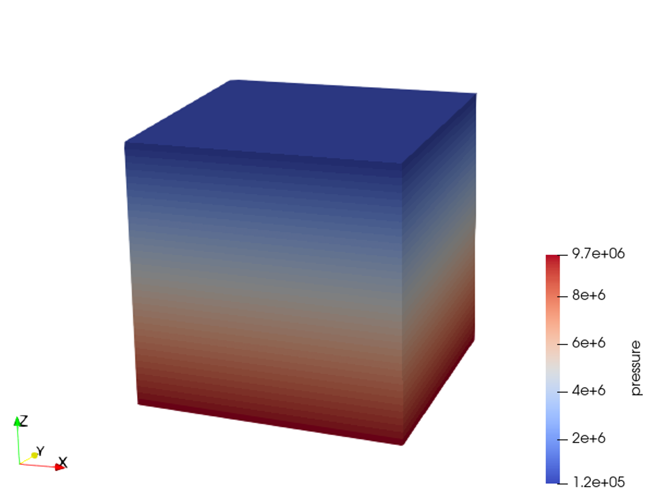
Fig. 94 Simulation result of pressure
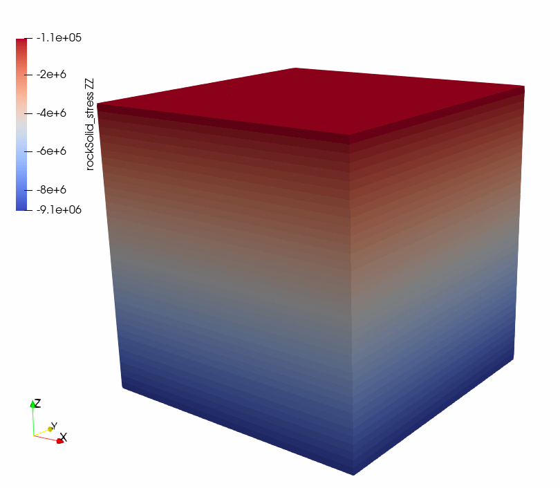
Fig. 95 Simulation result of effective vertical stress
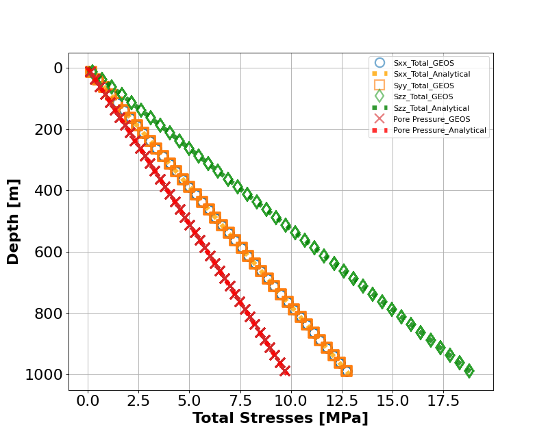
The figure below shows the comparison between the total stress computed by GEOS(marks) and with an analytical solutions (solid lines). Note that, because of the use of an isotropic model, the minimum and maximul horizontal stresses are equal.
To go further
Feedback on this example
For any feedback on this example, please submit a GitHub issue on the project’s GitHub page.