Toughness dominated KGD hydraulic fracture¶

Description of the case¶

In this example, we consider a plane-strain hydraulic fracture propagating in an infinite, homogeneous and elastic medium, due to fluid injection at a rate $Q_0$ during a period from 0 to $t_{max}$ . Two dimensional KGD fracture is characterized as a vertical fracture with a rectangle-shaped cross section. For verification purpose, the presented numerical model is restricted to the assumptions used to analytically solve this problem (Bunger et al., 2005). Vertical and impermeable fracture surface is assumed, which eliminate the effect of fracture plane inclination and fluid leakoff. The injected fluid flows within the fracture, which is assumed to be governed by the lubrication equation resulting from the mass conservation and the Poiseuille law. Fracture profile is related to fluid pressure distribution, which is mainly dictated by fluid viscosity $\mu$ . In addition, fluid pressure contributes to the fracture development through the mechanical deformation of the solid matrix, which is characterized by rock elastic properties, including the Young modulus $E$ , and the Poisson ratio $\nu$ .

For toughness-dominated fractures, more work is spent to split the intact rock than that applied to move the fracturing fluid. To make the case identical to the toughness dominated asymptotic solution, incompressible fluid with an ultra-low viscosity of 0.001 cp and medium rock toughness should be defined. Fracture is propagating with the creation of new surface if the stress intensity factor exceeds rock toughness $K_{Ic}$ .

In toughness-storage dominated regime, asymptotic solutions of the fracture length $\ell$ , the net pressure $p_0$ and the fracture aperture $w_0$ at the injection point for the KGD fracture are provided by (Bunger et al., 2005):

$\ell = 0.9324 X^{ -1/6 } (\frac{ E_p Q_0^3 }{ 12\mu })^{ 1/6 } t^{ 2/3 } w_0^2 = 0.5 X^{ 1/2 } (\frac{ 12\mu Q_0 }{ E_p })^{ 1/2 } \ell w_0 p_0 = 0.125 X^{ 1/2 } (12\mu Q_0 E_p)^{ 1/2 }$

where the plane modulus $E_p$ is defined by

$E_p = \frac{ E }{ 1-\nu^2 }$

and the term $X$ is given as:

$X = \frac{ 256 }{ 3 \pi^2 } \frac{ K_{Ic}^4 }{ \mu Q_0 {E_p}^3 }$

Input file

The xml input files for this test case are located at:

inputFiles/hydraulicFracturing/kgdToughnessDominated_base.xml

and

inputFiles/hydraulicFracturing/kgdToughnessDominated_benchmark.xml

The corresponding integrated test with coarser mesh and smaller injection duration is also prepared:

inputFiles/hydraulicFracturing/kgdToughnessDominated_Smoke.xml

Mechanics solvers¶

The solver SurfaceGenerator defines rock toughness $K_{Ic}$ as:

    <SurfaceGenerator
      name="SurfaceGen"
      targetRegions="{ Domain }"
      nodeBasedSIF="1"
      solidMaterialNames="{ rock }"
      rockToughness="1e6"
      mpiCommOrder="1"/>

Rock and fracture deformation are modeled by the solid mechanics solver SolidMechanicsLagrangianSSLE. In this solver, we define targetRegions that includes both the continuum region and the fracture region. The name of the contact constitutive behavior is also specified in this solver by the contactRelationName, besides the solidMaterialNames.

    <SolidMechanicsLagrangianSSLE
      name="lagsolve"
      timeIntegrationOption="QuasiStatic"
      discretization="FE1"
      targetRegions="{ Domain, Fracture }"
      solidMaterialNames="{ rock }"
      contactRelationName="fractureContact"/>

The single phase fluid flow inside the fracture is solved by the finite volume method in the solver SinglePhaseFVM as:

    <SinglePhaseFVM
      name="SinglePhaseFlow"
      discretization="singlePhaseTPFA"
      targetRegions="{ Fracture }"
      fluidNames="{ water }"
      solidNames="{ fractureFilling }"
      permeabilityNames="{ fracturePerm }"/>

All these elementary solvers are combined in the solver Hydrofracture to model the coupling between fluid flow within the fracture, rock deformation, fracture opening/closure and propagation. A fully coupled scheme is defined by setting a flag FIM for couplingTypeOption.

    <Hydrofracture
      name="hydrofracture"
      solidSolverName="lagsolve"
      fluidSolverName="SinglePhaseFlow"
      surfaceGeneratorName="SurfaceGen"
      porousMaterialNames="{ fractureFilling }"
      couplingTypeOption="FIM"
      logLevel="1"
      discretization="FE1"
      targetRegions="{ Fracture }"
      contactRelationName="fractureContact"
      maxNumResolves="2">

The constitutive laws¶

The constitutive law CompressibleSinglePhaseFluid defines the default and reference fluid viscosity, compressibility and density. For this toughness dominated example, ultra low fluid viscosity is used:

    <CompressibleSinglePhaseFluid
      name="water"
      defaultDensity="1000"
      defaultViscosity="1.0e-6"
      referencePressure="0.0"
      compressibility="5e-10"
      referenceViscosity="1.0e-6"
      viscosibility="0.0"/>

The isotropic elastic Young modulus and Poisson ratio are defined in the ElasticIsotropic block. The density of rock defined in this block is useless, as gravity effect is ignored in this example.

    <ElasticIsotropic
      name="rock"
      defaultDensity="2700"
      defaultYoungModulus="30.0e9"
      defaultPoissonRatio="0.25"/>

Mesh¶

Internal mesh generator is used to generate the geometry of this example. The domain size is large enough comparing to the final size of the fracture. A sensitivity analysis has shown that the domain size in the direction perpendicular to the fracture plane, i.e. x-axis, must be at least ten times of the final fracture half-length to minimize the boundary effect. However, smaller size along the fracture plane, i.e. y-axis, of only two times the fracture half-length is good enough. It is also important to note that at least two layers are required in z-axis to ensure a good match between the numerical results and analytical solutions, due to the node based fracture propagation criterion. Also in x-axis, bias parameter xBias is added for optimizing the mesh by refining the elements near the fracture plane.

Defining the initial fracture¶

The initial fracture is defined by a nodeset occupying a small area where the KGD fracture starts to propagate:

    <Box
      name="fracture"
      xMin="{ -0.01, -0.01, -0.01 }"
      xMax="{  0.01,  1.01,  1.01 }"/>

This initial ruptureState condition must be specified for this area in the following FieldSpecification block:

    <FieldSpecification
      name="frac"
      initialCondition="1"
      setNames="{ fracture }"
      objectPath="faceManager"
      fieldName="ruptureState"
      scale="1"/>

Defining the fracture plane¶

The plane within which the KGD fracture propagates is predefined to reduce the computational cost. The fracture plane is outlined by a separable nodeset by the following initial FieldSpecification condition:

    <Box
      name="core"
      xMin="{ -0.01, -0.01, -0.01 }"
      xMax="{  0.01, 50.01,  1.01 }"/>

    <FieldSpecification
      name="separableFace"
      initialCondition="1"
      setNames="{ core }"
      objectPath="faceManager"
      fieldName="isFaceSeparable"
      scale="1"/>

Defining the injection rate¶

Fluid is injected into a sub-area of the initial fracture. Only half of the injection rate is defined in this boundary condition because only half-wing of the KGD fracture is modeled regarding its symmetry. Hereby, the mass injection rate is actually defined, instead of the volume injection rate. More precisely, the value given for scale is $Q_0 \rho_f/2$ (not $Q_0 /2$ ).

The parameters used in the simulation are summarized in the following table.

Symbol Parameter Units Value

$Q_0$ Injection rate [m:sup:3/s] 10:sup:-4

$E$ Young’s modulus [GPa] 30

$\nu$ Poisson’s ratio [ - ] 0.25

$\mu$ Fluid viscosity [Pa.s] 10:sup:-6

$K_{Ic}$ Rock toughness [MPa.m:sup:1/2] 1

Inspecting results¶

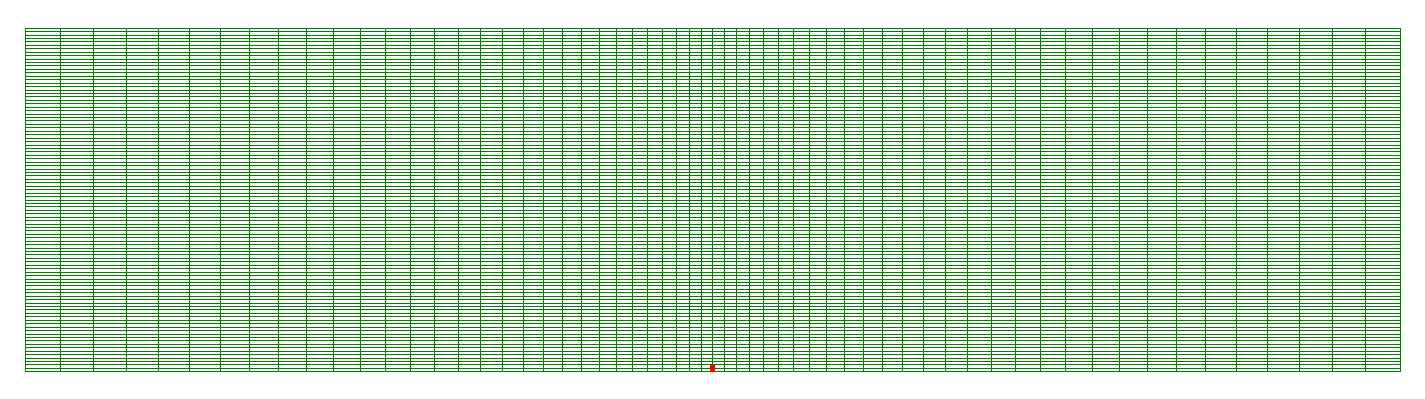
Fracture propagation during the fluid injection period is shown in the figure below.

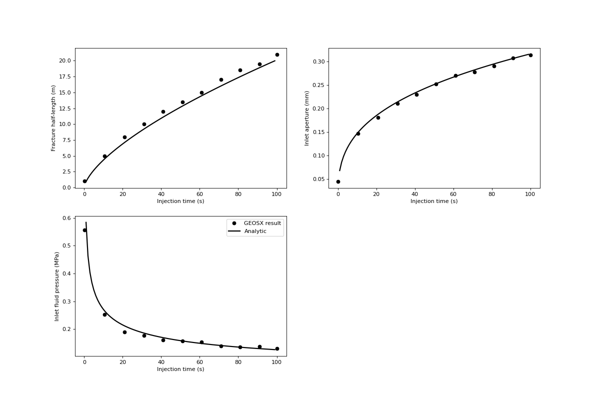
A good agreement between GEOSX results and analytical solutions is shown in the comparison below:

(Source code)

../../../../../_images/Example-1_01_006.png

To go further¶

Feedback on this example

This concludes the toughness dominated KGD example. For any feedback on this example, please submit a GitHub issue on the project’s GitHub page.