Sneddon’s Problem¶

Objectives

At the end of this example you will know:

how to define embedded fractures in the porous domain,

how to use the SolidMechanicsEmbeddedFractures solver to solve mechanics problems with embedded fractures.

Input file

This example uses no external input files and everything required is contained within a single GEOSX input file. The xml input file for this test case is located at:

src/coreComponents/physicsSolvers/solidMechanics/benchmarks/Sneddon-Validation.xml

Description of the case¶

We compute the displacement field induced by the presence of a pressurized fracture, of length $L_f$ , in a porous medium.

GEOSX will calculate the displacement field in the porous matrix and the displacement jump at the fracture surface. We will use the analytical solution for the fracture aperture, $w_n$ (normal component of the jump) to, i.e.

$w_n (s) = \frac{4(1 - \nu^2)p_f}{E} \, \sqrt{ \frac{L_f^2}{4} - s^2 }$

where - $E$ is the Young’s modulus - $\nu$ is the Poisson’s ratio - $p_f$ is the fracture pressure - $s$ is the local fracture coordinate in $[-\frac{L_f}{2}, \frac{L_f}{2}]$

All inputs for this case are contained inside a single XML file. In this example, we focus our attention on the Solvers tags, the ElementRegions tags and the Geometry tags.

Embedded fractures mechanics solver¶

To define a mechanics solver capable of including embedded fractures, we will define two solvers:

a SolidMechanicsEmbeddedFractures solver, called mechSolve

a small-strain Lagrangian mechanics solver, of type SolidMechanicsLagrangianSSLE called here matrixSolver (see: Solid Mechanics Solver)

Note that the name attribute of these solvers is chosen by the user and is not imposed by GEOSX. It is important to make sure that the solidSolverName specified in the embedded fractures solver corresponds to the small-strain Lagrangian solver used in the matrix.

The two single-physics solvers are parameterized as explained in their respective documentation, each with their own tolerances, verbosity levels, target regions, and other solver-specific attributes.

Additionally, we need to specify another solver of type, EmbeddedSurfaceGenerator, which is used to discretize the fracture planes.

    <SolidMechanicsEmbeddedFractures
      name="mechSolve"
      targetRegions="{ Domain, Fracture }"
      fractureRegionName="Fracture"
      initialDt="10"
      solidSolverName="matrixSolver"
      contactRelationName="fractureContact"
      logLevel="1">
      <NonlinearSolverParameters
        newtonTol="1.0e-6"
        newtonMaxIter="2"
        maxTimeStepCuts="1"/>
      <LinearSolverParameters
        directParallel="0"/>
    </SolidMechanicsEmbeddedFractures>

    <SolidMechanicsLagrangianSSLE
      name="matrixSolver"
      timeIntegrationOption="QuasiStatic"
      logLevel="1"
      discretization="FE1"
      targetRegions="{ Domain }"
      solidMaterialNames="{ rock }"/>

    <EmbeddedSurfaceGenerator
      name="SurfaceGenerator"
      solidMaterialNames="{ rock }"
      targetRegions="{ Domain, Fracture }"
      fractureRegion="Fracture"
      logLevel="1"/>
  </Solvers>

Events¶

For this problem we will add two events defining solver applications:

an event specifying the execution of the EmbeddedSurfaceGenerator to generate the fracture elements.
a periodic even specifying the execution of the embedded fractures solver.

  <Events
    maxTime="10">
    <SoloEvent
      name="preFracture"
      target="/Solvers/SurfaceGenerator"/>

    <PeriodicEvent
      name="solverApplications"
      forceDt="10"
      target="/Solvers/mechSolve"/>

Mesh, material properties, and boundary conditions¶

Last, let us take a closer look at the geometry of this simple problem. We use the internal mesh generator to create a large domain ( $1000\, m \, \times 1001 \, m \, \times 1 \, m$ ), with one single element along the Z axes, 420 elements along the X axis and 121 elements along the Y axis. All the elements are hexahedral elements (C3D8) and that refinement is performed around the fracture.

  <Mesh>
    <InternalMesh
      name="mesh1"
      elementTypes="{ C3D8 }"
      xCoords="{ 0, 400, 600, 1000 }"
      yCoords="{ 0, 400, 601, 1001 }"
      zCoords="{ 0, 100 }"
      nx="{ 10, 400, 10 }"
      ny="{ 10, 101, 10 }"
      nz="{ 1 }"
      cellBlockNames="{ cb1 }"/>
  </Mesh>

The parameters used in the simulation are summarized in the following table.

Symbol Parameter Units Value

$E$ Young’s modulus [Pa] 10⁴

$\nu$ Poisson’s ratio [-] 0.2

$L_f$ Fracture length [m] 20

$p_f$ Fracture pressure [Pa] 10⁵

Material properties and boundary conditions are specified in the Constitutive and FieldSpecifications sections.

Adding an embedded fracture¶

  <Geometry>
    <BoundedPlane
      name="FracturePlane"
      normal="{ 0, 1, 0 }"
      origin="{ 500, 500.5, 50 }"
      lengthVector="{ 1, 0, 0 }"
      widthVector="{ 0, 0, 1 }"
      dimensions="{ 20, 100 }"/>
  </Geometry>

Running GEOSX¶

To run the case, use the following command:

path/to/geosx -i src/coreComponents/physicsSolvers/solidMechanics/benchmarks/Sneddon-Validation.xml

Inspecting results¶

This plot compares the analytical pressure solution (continuous lines) at selected times with the numerical solution (markers).

../../../../../_images/Verification1.png

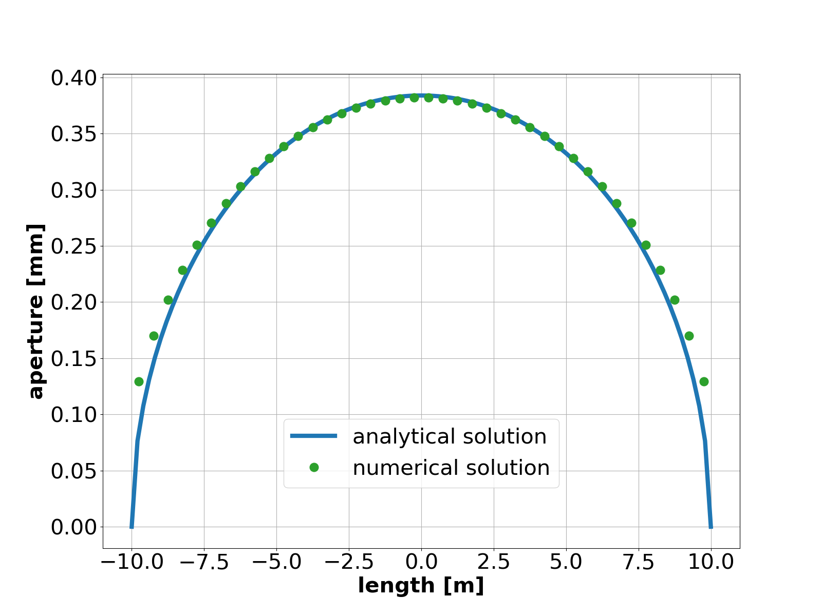
Fig. 2 Comparing GEOSX results with analytical solution

(Source code)

To go further¶

Feedback on this example

This concludes the Sneddon example. For any feedback on this example, please submit a GitHub issue on the project’s GitHub page.